Normal Distribution: Definition and Examples

Introduction:

A probability distribution is a function that gives the relationship between the outcome of a random variable in any random experiment and its probable values.

In this article, we will discuss one of the probability distributions which is commonly used in Data Science,

Normal Distribution or Gaussian Distribution.

To know more about Random Variable, read the article Introduction to Probability.

To know about other probability distributions, read the article Probability Distribution used in Data Science.

Table of Content:

• Normal Distribution
• Mathematical Definition
• Effect of Mean and Standard Deviation on Normal Distribution
• Properties of Normal Distribution
• Standard Normal Distribution

Normal Distribution:

Normal Distribution or Gaussian Distribution (named after German mathematician Carl Friedrich Gauss) is a continuous Probability distribution,

which is symmetric about its mean value (i.e. data near the mean value are more frequently occurring).

Example: 

• Height of Students in the school
• The score of the student in any exam.

Note: Normal distribution is often known as the bell-shaped curve.

Before going further let’s have an example.

Consider the experiment of Number of books read by students in a school

Mathematical Definition:

To know more about the mean, and variance read the article on Measures of Central Tendency and Measures of Dispersion.

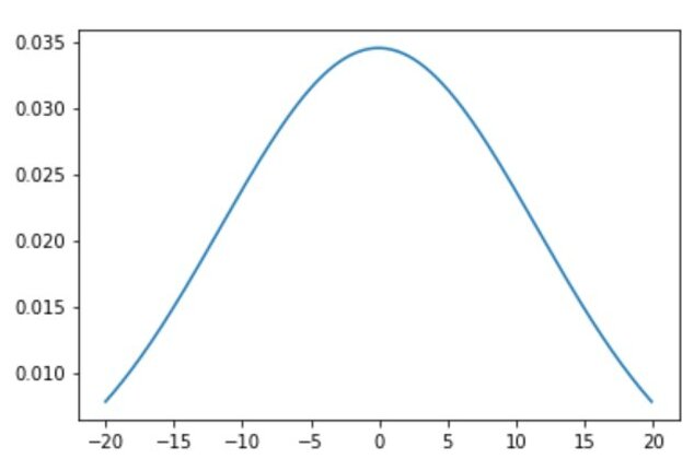
Example: Normal Distribution curve using Python

# importing libraries
 
import numpy as np
import matplotlib.pyplot as plt
import statistics as st
from scipy.stats import norm  #norm : normal distribution function
 
# distribution parameters
 
sample_set = np.arange(-20, 20, 0.1) 
#arange (start, stop, step-size): used to generate linear sequence with a constant step size
mean = st.mean(sample_set)
sd = st.stdev(sample_set)
 
# plot the normal distribution function with the defined mean and standard deviation
 
plt.plot(sample_set, norm.pdf(sample_set, mean, sd))

Effect of Mean and standard deviation on Normal Distribution:

Same Mean – Different Standard Deviation

# import libraries
 
import numpy as np
import matplotlib.pyplot as plt
from scipy.stats import norm
 
# distribution parameters
sample_set = np.arange(-20, 20, 0.1) 
#arange (start, stop, step-size): used to generate linear sequence with a constant step size
 
# define multiple normal distributions: same mean and different standard deviation
 
plt.plot(sample_set, norm.pdf(sample_set, 0, 1), label='μ: 0, σ: 1')
plt.plot(sample_set, norm.pdf(sample_set, 0, 1.5), label='μ:0, σ: 1.5')
plt.plot(sample_set, norm.pdf(sample_set, 0, 2), label='μ:0, σ: 2')
 
#add legend to plot
plt.legend()

From the above, we get, if we change the standard deviation keeping the mean constant the larger standard deviation will give a flatter curve.

Different Mean – Same Standard Deviation

#import libraries
 
import numpy as np
import matplotlib.pyplot as plt
from scipy.stats import norm
 
# distribution parameters
 
sample_set = np.arange(-20, 20, 0.1) 
#arange (start, stop, step-size): used to generate linear sequence with a constant step size
 
#define multiple normal distributions: different mean and same standard deviation
 
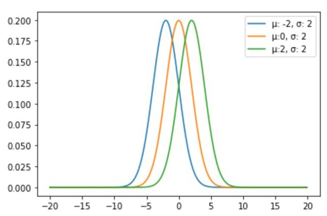
plt.plot(sample_set, norm.pdf(sample_set, -2, 2), label='μ: -2, σ: 2')
plt.plot(sample_set, norm.pdf(sample_set, 0, 2), label='μ:0, σ: 2')
plt.plot(sample_set, norm.pdf(sample_set, 2, 2), label='μ:2, σ: 2')
 
#add legend to plot
 
plt.legend()

From the above, we get if we change the mean, the curve will shift either on the right or the left side.

Properties of Normal Distribution:

• Symmetric The shape of the normal distribution is perfectly symmetric about the mean i.e. the equal number of observations lies on both sides of the mean.

• Mean = Median = Mode At the center of Normal distribution, all the measures of central tendency lie.

• The total area under the curve is 1.

• Empirical Rule:

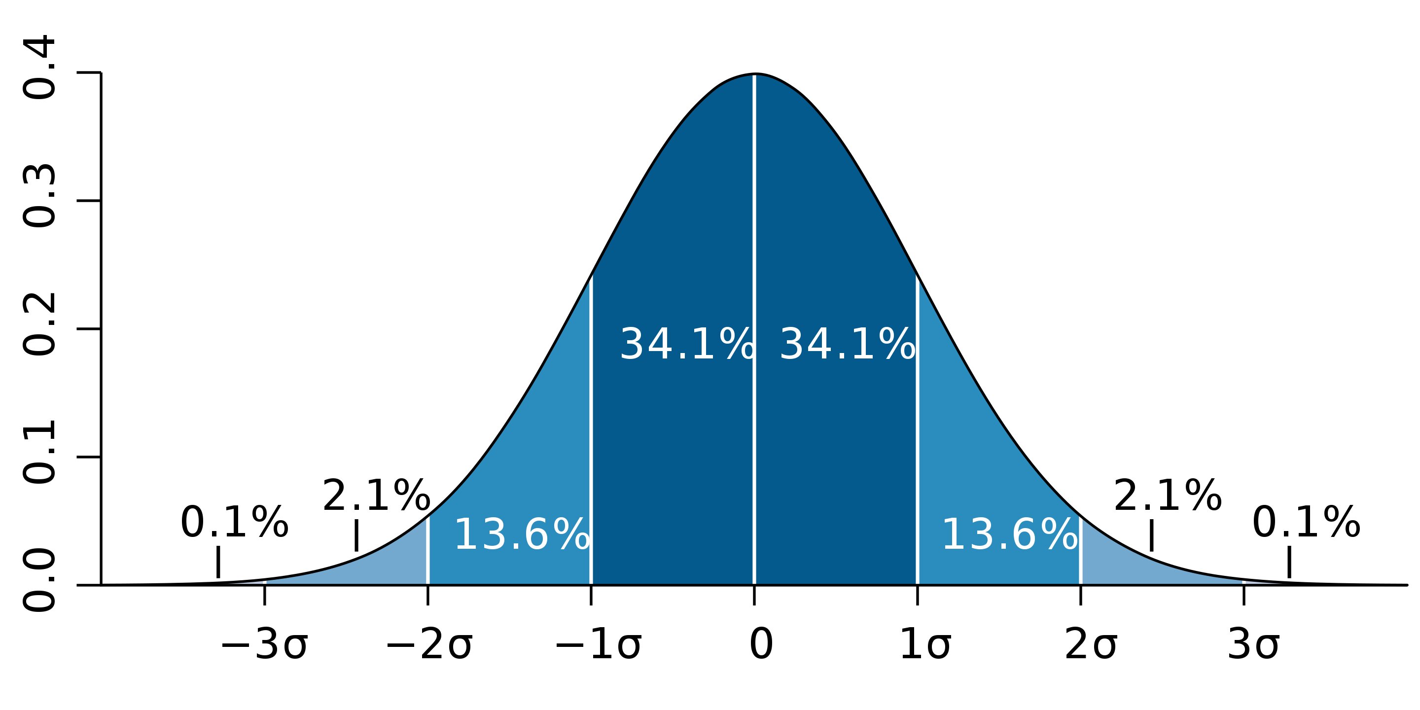
In a Normal Distribution, data is distributed in constant proportion, which is given by the Empirical rule.

The empirical rule or 68 – 95 – 97 rule or the Three sigma rule.

It states that in a Normal Distribution:

• 68% of the data will be within one Standard Deviation of the Mean
• 95% of the data will be within two Standard Deviations of the Mean
• 99.7 of the data will be within three Standard Deviations of the Mean

Standard Normal Distribution:

It is a special case of Normal Distribution for which mean = 0 and standard deviation = 1.

For any random variable X, Standard Normal Distribution is given by:

Conclusion:

In this article, we have discussed about one of the most important probability distribution Normal Distribution , with examples in python.

Hope this article will help in your data science and machine learning journey.

Top Trending Articles:
Data Analyst Interview Questions Data Science Interview Questions Machine Learning Applications Big Data vs Machine Learning Data Scientist vs Data Analyst How to Become a Data Analyst Data Science vs. Big Data vs. Data Analytics What is Data Science What is a Data Scientist What is Data Analyst