An Introduction to Principal Component Analysis

Principal Component Analysis (PCA) is one of the most popular statistical data extraction methods. PCA involves expressing a set of variables in a set of linear combinations of factors not correlated with each other. These factors account for an increasingly weak fraction of the variability of the data. PCA allows representing the original data (individuals and variables) in a space with a lower dimension than the original space while limiting the loss of information as much as possible. The representation of the data in spaces of weak dimension facilitates the analysis considerably.

PCA is mainly used to summarize the data structure described by various quantitative variables while acquiring factors that are not correlated with each other. These factors can be used as new variables that allow avoiding multicollinearity in multiple regression or discriminant factor analysis and carry out an automatic classification taking only essential information into account, which is, keeping only the first factors.

Must Read – Statistical Methods Every Data Scientist Should Know

Applications of Principal Component Analysis

• Reducing the size of the data space, making synthetic descriptions, and simplifying the problem under study
• Making representations of the original data in a space with a small dimension
• Transforming the correlated original variables into new uncorrelated variables that can be interpreted
• Dividing the experimental units into subgroups according to their similarity
• Transforming a set of correlated response variables into a set of uncorrelated components, under the criterion of maximum accumulated variability and, therefore, of minimum loss of information.
• Screening, which allows monitoring of the main components obtained to test hypotheses established in a multivariate data analysis study and to identify atypical data in the data set

You may also be interested in exploring: 

Popular Data Science Basics Online Courses & Certifications	Popular Machine Learning Online Courses & Certifications
Popular Deep Learning Online Courses & Certifications	Popular Python for data science Online Courses & Certifications

Steps of Principal Component Analysis

PCA mainly involves 5 crucial steps, explained below –

Standardize the Data Sets

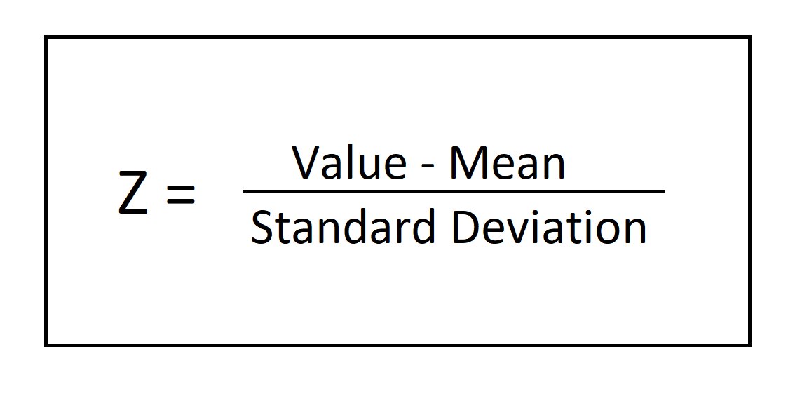
The PCA process identifies those directions in which the variance is greatest. As the variance of a variable is measured on, the same scale squared, if before calculating the components all the variables are not standardized so that they have a mean of 0 and a standard deviation of 1, those variables whose scale is larger will dominate the rest. Hence, it is advisable to always standardize the range of continuous initial variables.

You May Like  – ANOVA Test in Statistical Analysis – The Introduction

Calculate the Covariance Matrix 

A covariance matrix is a square matrix that shows the covariance between many different variables. Calculation of the covariance matrix helps to understand how the variables of the input data set are different from the mean or if any relationship exists between these variables. Most of the time variables are highly correlated which often results in them having redundant information, hence, to identify these correlations and redundancy, a covariance matrix needs to be calculated.

The formula to calculate the covariance matrix is as follows –

Compute the Eigenvectors and Eigenvalues of the Covariance Matrix

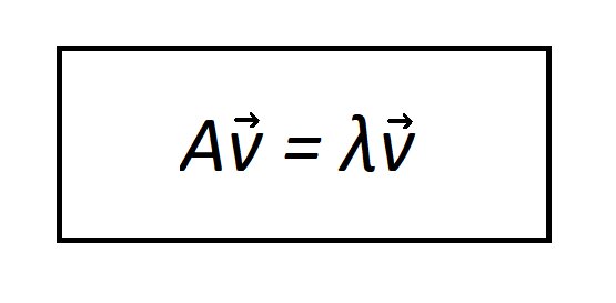
The eigenvectors or eigenvectors are the non-zero vectors of a linear map that, when transformed, give rise to a scalar multiple of them (they do not change direction). This scalar is the eigenvalue or eigenvalue and they help to identify the principal components.

Here is the calculation to find the eigenvalues ​​and eigenvectors associated with each eigenvalue of a matrix A.

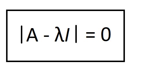
1. Calculate the roots of the characteristic polynomial of the matrix A. Said roots are the eigenvalues ​​of A. We must write down the algebraic multiplicity of each eigenvalue, that is, the number of times it appears as a solution in the characteristic polynomial.

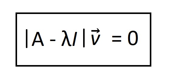
2. For each eigenvalue, we determine all non-trivial solutions for the following homogeneous system:

Where –

A = square matrix

v = vector

λ = scalar value

Notes on calculating eigenvalues ​​and eigenvectors in exercises

1. The eigenvalues or eigenvectors ​​can be complex numbers, It’s normal, don’t panic.
2. If A is an upper or lower triangular matrix or a diagonal matrix, the eigenvalues ​​of said matrix A are the elements of its main diagonal.
3. 0 is not considered the eigenvalue of A and neither is the null vector considered the eigenvector associated with the null eigenvalue.

Read More – Getting Started with Data Visualization: from Analysis to Aesthetics

Create a Feature Vector for Principal Component Analysis

Moving forward, PCA involves deciding which principal components to keep and which insignificant components (of low eigenvalues) to lose for creating a matrix of vectors, also called a Feature vector. This is the first step towards dimensionality reduction.

Recast the Data along the Principal Components Axes

We can now use the created feature vector to reorient the data from the original axes to the ones represented by the principal components. We can do this by multiplying the transposed original data set by the transposed row feature vector and completing the process of Principal Component Analysis.

If you have recently completed a professional course/certification, click here to submit a review.