Feature Selection in Machine Learning: Python code
Lets learn about feature selection in machine learning in detail with proper implementation in python.
The predictive accuracy of a machine learning model largely depends on its fed data. Hence, cleaning the data and selecting relevant features are the foremost important steps in model designing.
As a Data Scientist, one of the core practices you will be following is selecting value-adding features from a given data. By value-adding, we mean those features which will play a role in ensuring optimum performance of your machine learning model.
You must know that a model trains better on sizeable training data. While this holds for the number of records (rows) in a dataset, a higher number of features (columns) are often undesirable.
This article will discuss the concept of feature selection and the different techniques to select the best features for training a robust ML model. But before reading this article, I suggest you learn the basics of this article by reading Feature selection techniques. Beginners guide.
We will be covering the following section
3. Methods for Feature Selection
4. Performing Feature Selection Using Python
5. Endnotes
What is Feature Selection?
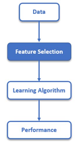
Feature Selection is a significant step in data pre-processing. It is also one of the main techniques in dimensionality reduction. Higher-dimensional data contains many redundant features that may negatively impact the performance of your model. Hence, it is important to identify ‘principal’ features from a dataset and filter out the irrelevant or unimportant features that will not contribute much to your target/prediction variable.
Best-suited Machine Learning courses for you
Learn Machine Learning with these high-rated online courses
Why Feature Selection?
1. Reduce model complexity
Data with fewer dimensions is computationally inexpensive and less complex. Also, the computational time reduces significantly as well.
2. Eliminate noise
Unrelated features add to the noise in data. Noisy data wreaks havoc on the entire ML pipeline. So, through feature selection, we minimize redundancy and maximize relevance to the target variable.
3. Improve model performance
As stated above, feature selection helps the model learn better. Properly trained models are more generalized as they alleviate the problem of overfitting.
Learn more about Overfitting and Underfitting with a real-life example


Methods for Feature Selection
There are various methods for performing feature selection on a dataset. We will discuss here the most important supervised feature selection methods that make use of output class labels. These methods use the target variable to identify relevant features that improve model accuracy.
Filter Methods
A feature can be regarded as irrelevant and discarded if it is conditionally independent of the class labels.
- Filter methods are generally used as a pre-processing step. These methods filter and select a subset of the data that contains only the relevant features.
- All features are ranked from best to worst based on the intrinsic properties of the data, such as correlation to the target variable, etc.
- Different filter methods, including the Chi-Square Test, ANOVA Test, Linear Discriminant Analysis (LDA), etc., use other criteria to measure the relevance of features.
- These methods are not dependent on the learning algorithm.
Wrapper Methods
- Simple methods have the same objective as filter methods but use an ML algorithm as their evaluation criterion.
- Data is divided into a feature subset that is fed to the learning algorithm. Based on how the model performs, we decide whether to add or remove features from the subgroup and train the model again to increase its accuracy.
- These methods produce more accurate models than filtering but consume a lot of computational resources and are usually slow to run.
- Famous examples include Forward Selection, Backwards Elimination, Recursive Feature Elimination (RFE), etc.
Note: Wrapper and Filter Methods are discrete processes, meaning the features are either kept or discarded. This can often cause high variance.
Embedded Methods
Embedded methods fuse the advantages of both filter and wrapper methods.
These methods perform feature selection and algorithm training in parallel. They are implemented by algorithms that have their integral feature selection process.
They are continuous methods and thus, don’t suffer much from high variability.
Examples of these methods are RIDGE and LASSO regression, which have built-in functions to help reduce overfitting.
Also explore:Ridge Regression vs Lasso Regression
Performing Feature Selection Using Python
Problem Statement:
For demonstration, we are going to make use of the Breast Cancer dataset from Kaggle to try and predict if the tumor is cancerous or not by looking at the given features. While doing so, we will use different feature selection techniques to see how it affects the training time and overall accuracy of a Random Forest Classifier model.
Let’s get started!
Dataset Description:
- ID number
- Diagnosis – Diagnosis of breast cancer (M = malignant, B = benign)
- radius (mean of distances from the center to points on the perimeter)
- texture (standard deviation of gray-scale values)
- perimeter
- area
- smoothness (local variation in radius lengths)
- compactness (perimeter^2 / area – 1.0)
- concavity (severity of concave portions of the contour)
- concave points (number of concave portions of the contour)
- symmetry
- fractal dimension (“coastline approximation” – 1)
The mean, standard error, and “worst” (mean of the three largest values) of the above features were computed for each image, resulting in 30 features.
All feature values are recoded with four significant digits.
Missing attribute values: none.
Target variable class distribution: 357 benign, 212 malignant.
Tasks to be performed:
1) Load the data
2) Get the list of features
3) Find correlation between features
4) Feature Selection with Correlation and Random Forest Classification
5) Recursive Feature Elimination (RFE) and Random Forest Classification
6) RFE with Cross-Validation and Random Forest Classification
7) Tree-Based Feature Selection and Random Forest Classification
Step 1 – Load the data
#Import required librariesimport timeimport numpy as np import pandas as pd import matplotlib.pyplot as pltfrom matplotlib.pyplot import figureimport seaborn as sns #Load the datadata = pd.read_csv('data.csv')data.head()
From our dataset displayed above, we can remove a few irrelevant features right away:
Ø The target variable ‘diagnosis’ should be separated from the feature set.
Ø The ‘id’ column is unnecessary for classification.
Ø The ‘Unnamed: 32’ column includes NaN values so we do not need it.
Step 2 – Get the list of features
#Get feature namescol = data.columns print(col) #Target variabley = data.diagnosis # M or B #Featureslist = ['Unnamed: 32','id','diagnosis']x = data.drop(list,axis = 1 )x.head() #Visualize the class labelsax = sns.countplot(y,label="Count") # M = 212, B = 357B, M = y.value_counts()print('Number of Benign: ',B)print('Number of Malignant : ',M)
Step 3 – Find correlation between features
#Correlation mapf,ax = plt.subplots(figsize=(18, 18))sns.heatmap(x.corr(), annot=True, linewidths=.5, fmt= '.1f',ax=ax)
The heat map displayed below visualizes the correlation between all of the features. Now, let’s get into the actual feature selection part!
Step 4 – Feature Selection with Correlation and Random Forest Classification
- According to the heat map we created above, we can infer the following:
- The features radius_mean, perimeter_mean, and area_mean are highly correlated with each other, so we will use only the area_mean feature.
- Similarly, the features compactness_mean, concavity_mean, and concave points_mean are correlated with each other. Therefore, we will choose only concavity_mean.
- The features radius_se, perimeter_se, and area_se are correlated, so we will use area_se.
- The features radius_worst, perimeter_worst, and area_worst are correlated, so we will use area_worst.
- The features compactness_worst, concavity_worst, and concave points_worst are correlated. So, we will use concavity_worst.
- The features compactness_se, concavity_se, and concave points_se are correlated. So, we will use concavity_se.
- The features texture_mean and texture_worst are correlated. So, we will use texture_mean.
- The features area_worst and area_mean are correlated, we will use area_mean.
drop_list1 = ['perimeter_mean','radius_mean','compactness_mean','concave points_mean','radius_se','perimeter_se','radius_worst','perimeter_worst', 'compactness_worst','concave points_worst','compactness_se','concave points_se','texture_worst','area_worst'] x_1 = x.drop(drop_list1,axis = 1 )x_1.head() After dropping features, we will create a correlation matrix again as shown below:#Correlation heatmapf,ax = plt.subplots(figsize=(14, 14))sns.heatmap(x_1.corr(), annot=True, linewidths=.5, fmt= '.1f',ax=ax)
As it can be seen in the above heatmap, no more highly correlated features. Actually, there is a correlation value of 0.9 but let’s see together what happens if we do not drop it.
So, we have chosen our features, but did we choose correctly? This will be answered by the performance of our Random Forest classifier.
Let’s split our data into 70% training and 30% testing set:
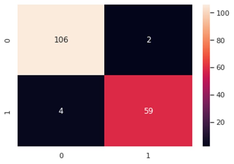
from sklearn.model_selection import train_test_split #Split the datax_train, x_test, y_train, y_test = train_test_split(x_1, y, test_size=0.3, random_state=42)Now, let’s train our classifier and find its accuracy score:from sklearn.ensemble import RandomForestClassifierfrom sklearn.metrics import f1_score,confusion_matrixfrom sklearn.metrics import accuracy_score #Build a random forest classifier with n_estimators=10 (default)clf_rf = RandomForestClassifier(random_state=43) clr_rf = clf_rf.fit(x_train,y_train) ac = accuracy_score(y_test,clf_rf.predict(x_test))print('Accuracy is: ',ac)cm = confusion_matrix(y_test,clf_rf.predict(x_test))sns.heatmap(cm,annot=True,fmt="d")
The accuracy is almost 96% and as can be seen in the confusion matrix, we do make a few wrong predictions. So, let’s try other feature selection methods to see if we find more accurate results.
Step 5 – Recursive Feature Elimination (RFE) and Random Forest Classification
from sklearn.feature_selection import RFE #Create the RFE objectclf_rf_2 = RandomForestClassifier() rfe = RFE(estimator=clf_rf_2, n_features_to_select=5, step=1)rfe = rfe.fit(x_train, y_train) print('Chosen best 5 feature by rfe:',x_train.columns[rfe.support_]) Let’s calculate the accuracy score of the Random Forest classifier when we use only the 5 selected features:x_train_2 = select_feature.transform(x_train)x_test_2 = select_feature.transform(x_test) #Random forest classifier with n_estimators=10 (default)clf_rf_2 = RandomForestClassifier() clr_rf_2 = clf_rf_2.fit(x_train_2,y_train) ac_2 = accuracy_score(y_test,clf_rf_2.predict(x_test_2))print('Accuracy is: ',ac_2)cm_2 = confusion_matrix(y_test,clf_rf_2.predict(x_test_2))sns.heatmap(cm_2,annot=True,fmt="d")
In this technique, we need to intuitively choose the number of features (k) we will use. Let’s have the value of k=5. Now, which 5 features are to be used would be chosen by the RFE method:
The accuracy is almost 95% which is lesser than the previous feature selection method we used.
However, this might also be because of our chosen value of k. Maybe if we use the best 2 or best 15 features, we might get better accuracy. Therefore. Let’s determine the optimal number of features we need:
Step 6 – RFE with Cross-Validation and Random Forest Classification
The accuracy score is proportional to the number of correct classifications:
from sklearn.feature_selection import RFECV clf_rf_3 = RandomForestClassifier() rfecv = RFECV(estimator=clf_rf_3, step=1, cv=5,scoring='accuracy') #5-fold cross-validationrfecv = rfecv.fit(x_train, y_train) print('Optimal number of features :', rfecv.n_features_)print('Best features :', x_train.columns[rfecv.support_]) We now have a list of 15 best features to get the best accuracy score for our model. Let’s visualize the accuracy through a plot:#Plot number of features VS. cross-validation scoresplt.figure()plt.xlabel("Number of features selected")plt.ylabel("Cross validation score of number of selected features")plt.plot(range(1, len(rfecv.grid_scores_) + 1), rfecv.grid_scores_)plt.show()
Step 7 – Tree-Based Feature Selection in Random Forest Classification
clf_rf_4 = RandomForestClassifier() clr_rf_4 = clf_rf_4.fit(x_train,y_train)importances = clr_rf_4.feature_importances_std = np.std([tree.feature_importances_ for tree in clf_rf.estimators_], axis=0)indices = np.argsort(importances)[::-1] #Print the feature rankingprint("Feature ranking:") for f in range(x_train.shape[1]): print("%d. feature %d (%f)" % (f + 1, indices[f], importances[indices[f]])) Plot the feature importances list:plt.figure(1, figsize=(14, 13))plt.title("Feature importances")plt.bar(range(x_train.shape[1]), importances[indices], color="g", yerr=std[indices], align="center")plt.xticks(range(x_train.shape[1]), x_train.columns[indices],rotation=90)plt.xlim([-1, x_train.shape[1]])plt.show()
In the random forest classification method, there is a feature_importances attribute that defines the importance of the features. To use it, the features in the training data should not be correlated. Random Forest chooses randomly at each iteration; therefore, the sequence of feature importances list can change.
As you can see in the above plot, after the 6 best features, the importance of features decreases. Therefore, we can focus on these 6 features.
Endnotes
Finding the best features from a given data can help us extract valuable information and improve model performance in machine learning hence, feature selection is a must-do step during any model building process. Artificial Intelligence & Machine Learning is an increasingly growing domain that has hugely impacted big businesses worldwide.


