How to Improve the Accuracy of Regression Model?

In this article, we will discuss how to improve accuracy of regression model with the help of simple examples to understand the concepts.

Introduction

Companies use various machine learning models as a basis to make major business decisions, and therefore the accuracy of a model is important. More effective, robust, and reliable the ML model is, the more profitable it is for businesses. It can produce more accurate predictions and insights, which deliver more business value and less errors. In this article, let’s go through various ways to improve the accuracy of a regression model.

A few effective ways to improve the accuracy of your regression models are:

1. Regularization
2. Handling Missing & Null Values
   1. Deleting Missing Values
   2. Imputing Missing Values
   3. Imputing by Model-based Prediction
3. Categorical Feature Encoding
   1. Label Encoding
   2. One-Hot Encoding
4. Feature Engineering
5. Conclusion

Regularization

One of the most common problems that you will come across when training your model is overfitting. A regression model is said to be overfitting when your algorithm is too complex, in a way that it fits the training data exceptionally well but fails to generalize the data that contains a lot of irrelevant data points. As in, the algorithm fits a limited set of data points very closely, thereby learning from noise in the data. This impacts the accuracy of the model. One of the ways of avoiding overfitting is using regularization.

In general, regularization simply means making something regular or acceptable. In machine learning regularization is a form of regression that shrinks (regularizes) coefficient estimates to zero. You can simply think of it as a damper that will repress the extra weights on special features in your algorithm and redistribute them evenly. This way regularization prevents overfitting by discouraging the learning of a model of both high complexity and flexibility. Mainly, there are two types of regularization techniques: Lasso Regression, Ridge Regression.

Must Check: What is Machine Learning?

Must Check: Machine Learning Online Course & Certification

It is a useful technique to improve the accuracy of your models. A popular Python library for implementing these algorithms is Scikit-Learn. Let’s try to learn this with the help of an example. First let’s import the libraries that we would require.

import numpy as np
from sklearn.datasets import make_regression
import pandas as pd
import matplotlib.pyplot as plt

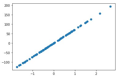
Usually samples are made from a smaller portion of the population. In some cases this can be heavily skewed leading to overfitting of a linear model.

X_sample,y_sample = make_regression(n_samples = 100,n_features = 1,noise=0.5)
 
#defines the sample taken from the population which is screwed
plt.scatter(X_sample,y_sample)
plt.show()

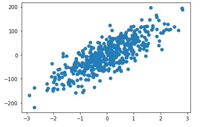
X_population, y_population = make_regression(n_samples=500,n_features=1,noise=40)
 
#this represents the entire population of true dataset
plt.scatter(X_population,y_population)
plt.show()

Now, let’s try to compare the accuracy of the model before and after regularization.

from sklearn.linear_model import LinearRegression
lr = LinearRegression().fit(X_sample,y_sample)
 
#overfitting
training_accuracy = lr.score(X_sample,y_sample)
print("training accuracy is: ",training_accuracy)

Output

#poor generalization
accuracy = lr.score(X_population,y_population)
print("accuracy on population is: ",accuracy)

Output

Let’s try to check the accuracy using the ridge and lasso regression techniques.

#now using ridge instead of normal linear regression 
from sklearn import linear_model
ridge = linear_model.Ridge(alpha=10)
ridge.fit(X_sample,y_sample)

training_ridge = ridge.score(X_sample,y_sample)
print("training accuracy with ridge ",training_ridge )

Output

accuracy_lasso = ridge.score(X_population,y_population)
print("accuracy with lasso: ",accuracy_lasso)

Output

As you can notice, regularization has increased the accuracy of generalization as it adds a penalty to the error. That said, it is important to correctly figure out which regularization technique works better for your model to get the accurate results.

Handling Missing and Null Values

Treating missing and null values in datasets is a crucial issue especially when you are dealing with complete available data. Properly handling missing data improves the inferences and the predictions made. A particular data element can be missing due to various reasons such as failure to load the information, corrupt data, incomplete load operations, etc.

Let us explore how to deal with missing & null values to improve the accuracy of the model.

To demonstrate this, we are going to use House_Price.csv, one of the popular Kaggle dataset used to predict sales prices and many other details. Let’s load the dataset as Pandas DataFrame.

The first step is to check and mark missing values as shown below.

# load the dataset and check for missing values
import pandas as pd
# load the dataset
dataset = pd.read_csv('house_price.csv')
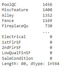
#check for missing values from each column
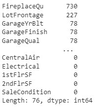
dataset.isnull().sum().sort_values(ascending=False)

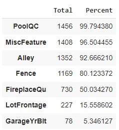
As you can see the dataset has plenty of columns with a huge amount of null values. Therefore to get the clear picture let us try to get the top 7 columns with higher percentage of null values.

totals = dataset.isnull().sum().sort_values(ascending=False)
percentage = totals/len(dataset)*100
pd.concat([totals,percentage], axis=1, keys=['Total','Percent']).head(7)

We clearly have 4 columns with Null values higher than 80%. So, how do you handle this missing data?

Deleting the Missing Values

One of the simple strategies for handling missing data is to delete those records from a dataset that contain missing values. While this method is not really recommended, you can use it when there are lots of missing values in a particular column and when you are dealing with a large amount of data.

Let us go ahead and delete columns with null values greater than 80%.

#Method 1: Removing columns with missing values > 80%
dataset = dataset[dataset.columns[dataset.isnull().mean() < 0.80]]
dataset.isnull().sum().sort_values(ascending=False)

When you completely get rid of data with missing values, the model is robust and accurate when the columns that you deleted do not have high weightage. However, if you remove those columns that have high correlation with output, then this method leads to less accuracy and loss of useful information.

Impute Missing Values

You can apply this strategy when you are dealing with features that have numeric data like age, salary, etc. There are various options that you can consider to replace the missing values.

• A mean, median, or mode for the column
• A random value from other randomly selected record
• Value from previous record or next record
• Most frequent value of that column

And many others. From the above dataset, we have a column called MSSubClass of integer type. In this column, let us replace the missing values with mean.

# Replacing missing values by the mean value 
dataset['MSSubClass'] = dataset['MSSubClass'].fillna(dataset['MSSubClass'].mean())
dataset['MSSubClass'].isnull().sum()

Imputing Missing Values for Categorical Features

In case of a non-numeric column, you cannot use mean or median. In such a case, you can replace the categorical features using the most frequent value or just treat it as a separate category. For example, let us replace the missing values of column FireplaceQu (FirePlace Quality) with the most frequent value.

# Before replacing - missing values count in FireplaceQu
dataset['FireplaceQu'].isnull().sum()

# Imputing missing values for categorical variable
dataset['FireplaceQu'] = dataset['FireplaceQu'].fillna(dataset['FireplaceQu'].mode()[0])
dataset['FireplaceQu'].isnull().sum()

Impute Missing Values with Model-based Prediction

In this model-based strategy, we use features which do not have null or missing values and train it to predict the missing values. This method gives us an advantage over replacing with median, mode, etc. This way of imputing missing data is more flexible.

What you are basically doing here is that, you are training your ML model to predict the missing values for a feature based on other features. The records (rows) without missing values are used as a training set and model also used values in other columns. You can use a classification or regression model to train based on the datatype of the feature. Post training, the model is then applied to samples with missing values to predict its most likely value.

Categorical Feature Encoding

Typically, a dataset has a combination of numerical and categorical values. However, most machine learning models work with numerical values only (or some other different values that are understandable to the ML model) and cannot operate on categorical data directly. This means that the categorical data has to be transformed to numerical form to be utilized by the algorithm. Categorical encoding is a data preparation technique that makes certain types of data readable by an algorithm and much easier to work with.

The three common categorical types of data are:

• Binary: a set of two values. Example: Pass or Fail
• Ordinal: a set of values in either ascending or descending order. Example: Rating from 1 to 10
• Nominal: a set of values with no particular order. Example: A list of cities

Based on the type of categorical type that you are handling, you can use Label Encoding or One-hot Encoding.

Label Encoding

Label encoding or integer encoding can be used when you are handling ordinal variables.

For example, “high” is 1, “medium” is 2, and “low” is 3.

Often the integer values start at 0 and by default the integers are assigned to labels in the order that they appear in the data. The integer values here have a natural ordered relationship between each other and hence the ML algorithm can easily understand and use this relationship. The integer encoding or ordinal encoding technique is easily reversible. Let’s learn more with the help of an example.

Our first step is to download the dataset and import required Python packages as shown below.

# load the dataset
import pandas as pd
dataset = pd.read_csv('healthcare-dataset-stroke-data.csv')
# print shape
print('data shape :', dataset.shape)

Let’s load the dataset and observe its shape. The above output indicates that we have 12 variables and 5110 rows.

Next, let us inspect a set of sample data using head().

#inspect data
dataset.head(5)

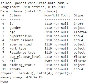
We can try to understand the dataset more by gathering some useful information using the info() method from pandas.

#Get information about the dataset
print(dataset.info())

The output above shows a list of features, size excluding null values, and data type for each variable. In the above example, we have around 5 features of object data type (most of them being categorical).

Let us now implement label encoding.

# Import the label encoder 
from sklearn import preprocessing
label_encoder = preprocessing.LabelEncoder()
# Transform column 'gender' (object type) to the numerical data type
dataset['gender']= label_encoder.fit_transform(dataset['gender']) 
dataset.head(5)

As you can see, the gender feature is now encoded to numerical data types, where 1 represents male and 0 represents female. Let us now try to encode. One problem is that label encoding might not be clear enough when you use it on variables where no ordinal relationship exists.

One-Hot Encoding

For categorical variables with no natural ordering or relationship between them, forcing an ordinal relationship via label encoding may result in poor performance or unexpected results. In such scenarios, one-hot encoding is useful. One-hot encoding converts each categorical value into a new categorical column and matches with binary values 0 & 1.

This technique is suitable when dealing with nominal variables.

One-Hot Encoding with Sklearn

Let us now learn how to implement one-hot encoding in Python with a simple example.

The first step is to define the data.

import pandas as pd
# create and define the data
# create DataFrame
dataf = pd.DataFrame({'Fruits': ['Apple', 'Mango', 'Banana', 'Apple', 'Orange', 'Orange'],
                   'Price': [85, 100, 50, 70, 60, 55]})
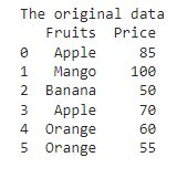
print("The original data")
print(dataf)

Next step is to perform one-hot encoding. To implement the one-hot encoding, you need to import the OneHotEncoder() function from sklearn library.

# importing OneHotEncoder
from sklearn.preprocessing import OneHotEncoder
# create an instance if one-hot encoder
encoder = OneHotEncoder(handle_unknown='ignore')
# encode the Fruits column
encoder_dataf = pd.DataFrame(encoder.fit_transform(dataf[['Fruits']]).toarray())
# merge encoded columns with the original column
final_dataf = dataf.join(encoder_dataf)
# rename the new columns if required
final_dataf.columns = ['Fruits', 'Price', 'Apple', 'Mango', 'Banana', 'Orange']
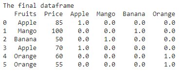
print("The final dataframe")
print(final_dataf)

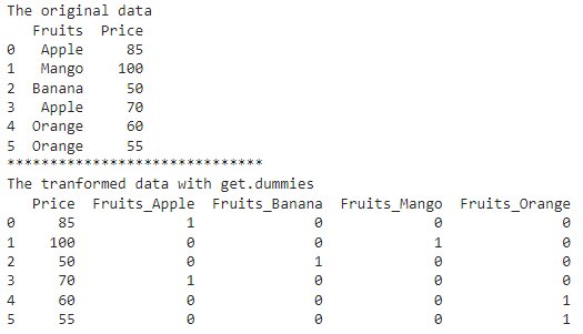
One-Hot Encoding Using Dummies Values Approach

Pandas, a popular Python library provides a function called get_dummies, using which you can enable one-hot encoding. This approach is more flexible as it allows you to encode as many category columns as required. You can also choose how to label the columns using a prefix.

import pandas as pd
import numpy as np
# create and define the data
# create DataFrame
dataf = pd.DataFrame({'Fruits': ['Apple', 'Mango', 'Banana', 'Apple', 'Orange', 'Orange'],
                   'Price': [85, 100, 50, 70, 60, 55]})
print("The original data")
print(dataf)
print("*" * 30)
# generate binary values using get_dummies function
encoder_dataf = pd.get_dummies(dataf, columns=["Fruits"])
print("The transformed data with get.dummies")
print(encoder_dataf)

Well, in the end it is important to know which encoding approach to use by being aware of its pros and cons.

Feature Engineering

Feature engineering is the process of using existing raw data & feature knowledge to formulate new useful features that better represent the underlying problem to predictive ML models. This inturn increases the accuracy of your model. As you might already know the features in your data will directly influence the model you use and the output that you achieve. Therefore, by creating good features you can augment the value of your existing data and thus improve the accuracy of your model.

Process that are involved in feature engineering are:

1. Feature Importance: Estimate usefulness of features
2. Feature Construction: Manually creating new features from raw data
3. Feature Extraction: Automated formulation of new features from raw data
4. Feature Transformations: Adjusting the features to improve the accuracy and performance of the model
5. Feature Selection: Select a subset of features that are important to model

Obviously, when you are working with real world data, it is too rare to get it accurate in the first iteration. Feature engineering is an iterative process, which might look as follows:

In the end, you need a well defined problem and domain knowledge to know when to stop this process and move on to trying other model configurations.

Conclusion

In this article we have discussed a few important ways to improve the accuracy of the regression model with the help of simple examples to understand the concept. Apart from what is discussed here, there are plenty other ways to improve the accuracy of your machine learning models. However, one important thing is that improving the accuracy of a ML model is a skill that you can master only with a lot of experimenting and practice.

Top Trending Articles:

Data Analyst Interview Questions | Data Science Interview Questions | Machine Learning Applications | Big Data vs Machine Learning | Data Scientist vs Data Analyst | How to Become a Data Analyst | Data Science vs. Big Data vs. Data Analytics | What is Data Science | What is a Data Scientist | What is Data Analyst