INDEX function in Excel

The INDEX function in Excel is a very powerful formula within the search and reference functions. The INDEX function is considered the predecessor of VLOOKUP and HLOOKUP. This function has two forms of use: Array and Reference.

What is the INDEX function in Excel?

The INDEX Function helps us find data or value within a range of cells or specified tables, allowing us to have the information at hand when it is required.

What it does:

• Returns the value at a given location within a specified range or array.
• Can extract single cells, entire rows, or columns of data.
• Can be used for lookups or to build dynamic formulas.

How to Use the INDEX function in Excel?

The INDEX Function searches within a table or range according to the row or column number we indicate (coordinates), a value or the reference of a value at the intersection of these.

There are two ways to use the INDEX Function, such as the Array Form and the Reference Form -

Array Form of the INDEX Function

The array form of the INDEX function is especially useful when you want to extract multiple values ​​from an array or range in a single formula. Instead of returning a single value, the array INDEX  function can return an array of results. This is possible by entering more than one row or column number as arguments.

The syntax of the matrix form is as follows:

=INDEX(array; row_num; [column_num])

The array form of the INDEX function has the following arguments:

• Array (required): The range of cells that comprise our data table.
• row_num (optional): The cell's row number containing the required value.
• column_num (optional): This argument is optional only if the Matrix consists of a single column. Otherwise, the column number of the searched cell must be specified.

Example - Use of the Array Form of the INDEX Function

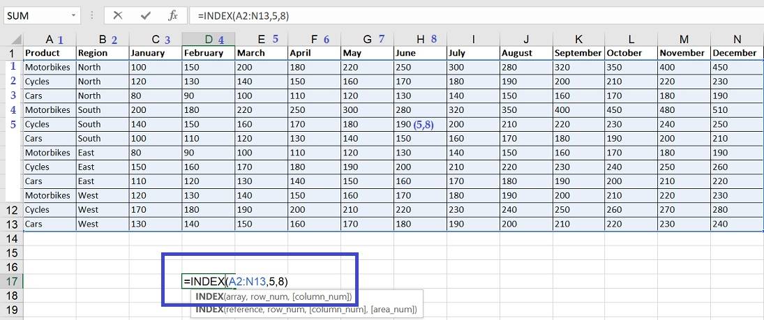
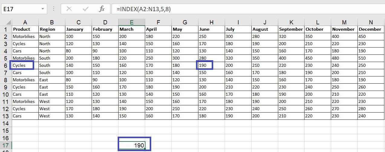
Let's say we want to extract the sales figures for "Cycle" in June. We can achieve this using the INDEX function's array form. We will use the below formula - 

=INDEX(A2:N13,5,8)

Explanation

• It extracts a value from a table (data_range) based on product and month.
• Imagine the table has product names as the first row and month names as the first column.
• product_row (here, 5) tells the formula which row to look in for the product ("Cycle").
• month_column (here, 8) tells the formula which column to look in for the month (June).
• The formula returns the value where those two meet (sales figure for "Cycle" in June).

Reference Form of the INDEX Function

The second way to use the INDEX function in Excel is similar to the previous one, but with the difference that instead of specifying a single matrix, we can indicate more than one matrix. This is useful when you only want to extract values ​​from a specific part of your data.

The syntax of the reference form is as follows:

=INDEX(ref, row_num, [column_num], [area_num])

The reference form of the INDEX function has the following arguments:

• Ref (required): The reference to the arrays that hold the data. Ref can specify multiple ranges, such as A2:N7, A8:N13
• row_num (required): The row number of the cell we want to obtain.
• column_num(optional): The column number of the cell to obtain.
• area_num (optional): Since Ref indicates which ranges should be used, we must mention the reference range we pick. Usually denoted as 1 or 2.

Example - Use of the Reference Form of the INDEX Function

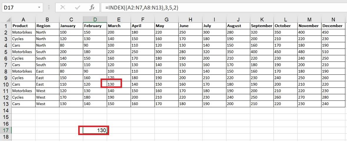
In this example, we want to extract the sales figures for "Cars" in March. We can achieve this using the INDEX function's reference form. We will use the below formula - 

=INDEX((A2:N7,A8:N13),3,5,2)

Explanation

The formula uses a combined range (A2:N7,A8:N13). This means it's looking at two separate ranges: A2:N7 and A8:N13.

• row_num (3): 3 specifies the row number but is now within the combined range.
• column_num (5): 5 specifies the column number within the chosen range (A8:N13 due to the tiebreaker).
• area_num: The third argument, 2, acts as a "tiebreaker" when using combined ranges. It tells the INDEX function to prioritise the second range (A8:N13) when there's a row match in both ranges at position 3.

It retrieves the value from the 3rd row and 5th column within the range A8:N13 (2). So, it essentially focuses on the second half of the data (rows 8-13). So after applying the formula, we get the result 130, which shows that based on the given data, "Car" had sales of 130 units in March.

Observations

1. If the row_num and column_num arguments are used, INDEX returns the cell's value at the intersection of the row_num and column_num arguments.
2. The row_num and column_num arguments must indicate a cell within the array; otherwise, INDEX returns a #REF!
3. If you set row_num or column_num to 0 (zero), INDEX returns the array of values ​​for the entire column or row, respectively. Write the INDEX function as an array formula to use the returned values ​​as an array.