Introduction to Seaborn Scatter Plot

When you are analyzing your data like a data scientist, you’re sure to perform Exploratory Data Analysis (EDA) on your data during the initial stages of data processing. EDA helps in understanding, analyzing, and condensing the main characteristics of your data through popular data visualization methods.

One such popular visualization method is the  Seaborn  library in Python. It is an extension to Python’s Matplotlib library and integrates very well with the Pandas data structure. It also offers an easy and intuitive data visualization. We are back with a tutorial on Scatter Plot using Seaborn. We have already learned Matplotlib Scatter Plot. 

In this blog, we will be covering the following sections: 

• Introduction to Scatter Plots in Seaborn 
• Installing and Importing Seaborn 
• Get the Seaborn Datasets 
• Creating a Seaborn Scatter Plot 
• Adding Elements to the Scatter Plot 
• Common Attributes of the Scatter Plot 

Introduction to Scatter Plot in Seaborn 

A scatter plot is used to obtain the correlational relationship between two numerical variables. The positioning of the data points, called markers, allows us to infer if there is a correlation between the variables. It also depicts the direction and the strength of this correlation.  

Installing and Importing Seaborn 

Firstly, we will install the Seaborn library in our working environment through the following command: 

pip install seaborn 

Now that we have installed Seaborn, let’s install the necessary packages and libraries that Seaborn is dependent on: 

• NumPy 
• Pandas 
• Matplotlib 
• SciPy 

Let’s import all the libraries we’re going to work with today: 

import seaborn as sns 
import numpy as np 
import pandas as pd 
import matplotlib.pyplot as plt 

Get the Seaborn Datasets 

The Seaborn library offers a list of datasets that can be used for plotting data using its powerful plotting functions. The following command will list them all down: 

#Datasets available in seaborn 
sns.get_dataset_names() 

Today, we are going to pick the ‘car_crashes’ dataset to understand how to visualize data using the Seaborn scatter plot. We are going to analyze the relationship between two numerical features.  

Creating a Seaborn Scatter Plot 

Loading the data 

#Load the data 
df = sns.load_dataset('car_crashes') 
df.head()

#Get column names and data types 
df.info() 

Except for the ‘abbrev’ column, the rest of the 7 columns are numerical features. Now, we are going to analyze this dataset through a scatter plot. 

Plotting the data 

Now, we’ll use the sns.scatterplot() function to plot a relationship between the total car crashes and the influence of alcohol: 

#Create Scatterplot 
sns.scatterplot(x='total',y='alcohol',data=df) 

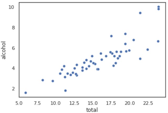
The above plot demonstrates that the columns ‘total’ and ‘alcohol’ are positively correlated, meaning the drivers with more alcohol in their systems tend to get into more car crashes. incur higher insurance costs. This pattern does make sense, right? Never drink and drive kids! 

Let’s label our plot for better readability.  

Adding Elements to the Scatter Plot 

As discussed above, because Seaborn is based on Matplotlib, different pyplot elements can be added to the plot to help ease its interpretation: 

• plt.title(): Used to specify a plot title 
• plt.xlabel() and plt.ylabel(): Used to label x and y-axis respectively 
• plt.show(): Used to display the plot 

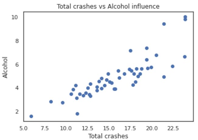
x = df['total'] 
y = df['alcohol'] 
 
#Add elements to scatterplot 
plt.scatter(x, y) 
plt.ylabel('Alcohol') 
plt.xlabel('Total crashes') 
plt.title('Total crashes vs Alcohol influence') 
plt.show() 

Common Attributes of the Scatter Plot 

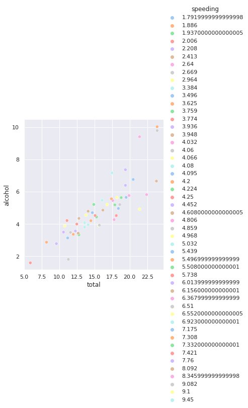
Hue parameter 

• You can use this attribute to group the data points with different colors. Let’s see how:  

#Add hue 
sns.scatterplot(x='total',y='alcohol',hue='speeding', data=df) 

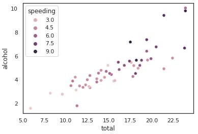
Can you observe how higher crashes and higher alcohol content are correlated to a higher speed? This is obvious as rash driving, drunk or not, often leads to accidents as well. 

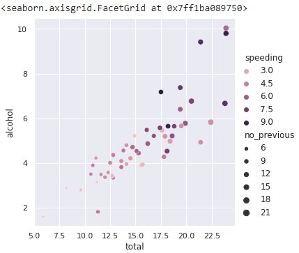
Size parameter 

• You can use the size parameter to group the data points with different sizes. Let’s see how:  

#Specify size parameter 
sns.scatterplot(x='total',y='alcohol',hue='speeding', size='no_previous',  data=df) 

One important point you should take note of is that the scatterplot() will produce the same result as relplot(kind=’scatter’) as it is the default plot in the relplot() function. 

So, we can also plot the above graph as – 

#relplot() function 
sns.relplot(x='total',y='alcohol',hue='speeding', size='no_previous', data=df

The lightest-colored data points seem to be fading in the white background. Let’s do something about it. 

Background theme and style  

• The set_theme() function sets the background theme for the plot. It can be set to one of the following options: 

(‘white’,’dark’,’whitegrid’,’darkgrid’,’ticks’) 

#Function - set_theme() 
sns.set_theme(style="darkgrid") 
sns.relplot(x='total',y='alcohol',hue='speeding', size='no_previous', data=df) 

Marker parameter 

• The default marker is a blue circle, as you have already seen in the above output. But the maskers are customizable. This is done by using the marker parameter to set marker types and style, as shown below: 

(‘v’, ’^’, ’>’, '<‘, ’o’, ’8′, ’s’, ’p’, ’*’, ’+’, ’h’, ’H’, ’D’, ’d’, ’P’, ’X’) 

#Change marker style 
sns.relplot(x='total',y='alcohol',hue='speeding', size='no_previous',  marker='v', data=df) 

Plot colors and palette parameter  

• The color_palette() function displays the colors currently present within Seaborn using the palplot() function: 

#Function – color_palette() 
snscolors = sns.color_palette() 
sns.palplot(snscolors) 

• The palette parameter is used to set colors to use for the different levels of the ’hue’ variable. It should be something that can be interpreted by color_palette(): 

#The palette parameter 
sns.relplot(x='total',y='alcohol',hue='speeding', palette='pastel', data=df)

Alpha parameter 

• You can use this attribute to set the transparency of markers between 0 and 1: 

#The alpha parameter 
sns.relplot(x='total',y='alcohol',hue='speeding', alpha=0.3, data=df) 

Endnotes 

A Scatter Plot is a very popular graph that you can use during data analysis. The Seaborn library is one of the most common libraries to create scatter plots. In fact, it is easier to customize and provides better functionality and organization capabilities than Matplotlib for basic plots. If you found this article informative, kindly leave a comment below.  

Interested in learning more about Python and Data Visualization? Explore related articles here. 

Top Trending Tech Articles:
Career Opportunities after BTech Online Python Compiler What is Coding Queue Data Structure Top Programming Language Trending DevOps Tools Highest Paid IT Jobs Most In Demand IT Skills Networking Interview Questions Features of Java Basic Linux Commands Amazon Interview Questions

Recently completed any professional course/certification from the market? Tell us what liked or disliked in the course for more curated content.

Click here to submit its review with Shiksha Online.