Movie Recommendation System using Machine Learning
Every time you open up YouTube just to figure out the solution to your problem or just get the latest news, you end up spending more time. A similar thing happens when you decided on binging through a single movie/series from an OTT you end up watching more than what you had in your mind. Ever wondered how they were able to do such a thing? Most of the OTT platforms depend on their movie recommendation system.
Contents
- But, what is a Recommendation System exactly?
- Why exactly do we need Recommendation Systems?
- Types of Recommendation Systems
But, what is a Recommendation System exactly?
A movie recommendation system is a fancy way to describe a process that tries to predict your preferred items based on your or people similar to you.
In layman’s terms, we can say that a Recommendation System is a tool designed to predict/filter the items as per the user’s behavior.
Best-suited Machine Learning courses for you
Learn Machine Learning with these high-rated online courses
Why exactly do we need Recommendation Systems?
From a user’s perspective, they are catered to fulfil the user’s needs in the shortest time possible. For example, the type of content you watch on Netflix or Hulu. A person who likes to watch only Korean drama will see titles related to that only but a person who likes to watch Action-based titles will see that on their home screen.
From an organization’s perspective, they want to keep the user as long as possible on the platform so that it will generate the most possible profit for them. With better recommendations, it creates positive feedback from the user as well. What good it will be to the organization to have a library of 500K+ titles when they cannot provide proper recommendations?
Recommendations are a great way to keep you watching but for Raghu the recommendations he gets wrong. But how? Well, as you know that recommendation systems are catered for a user but not for multiple users. Raghu lives in a joint family and everyone uses a single system to watch what they want. While OTT platforms give you a choice of adding multiple profiles but everyone else has already taken those and he is left with a single profile to share with his grandparents. So, Raghu decides to create his movie recommendation system. Before getting started he should understand the different types of recommendation systems.
Types of Recommendation Systems
The following figure shows different kinds of recommender systems:
Collaborative Filtering
There are two types of collaborative filtering:
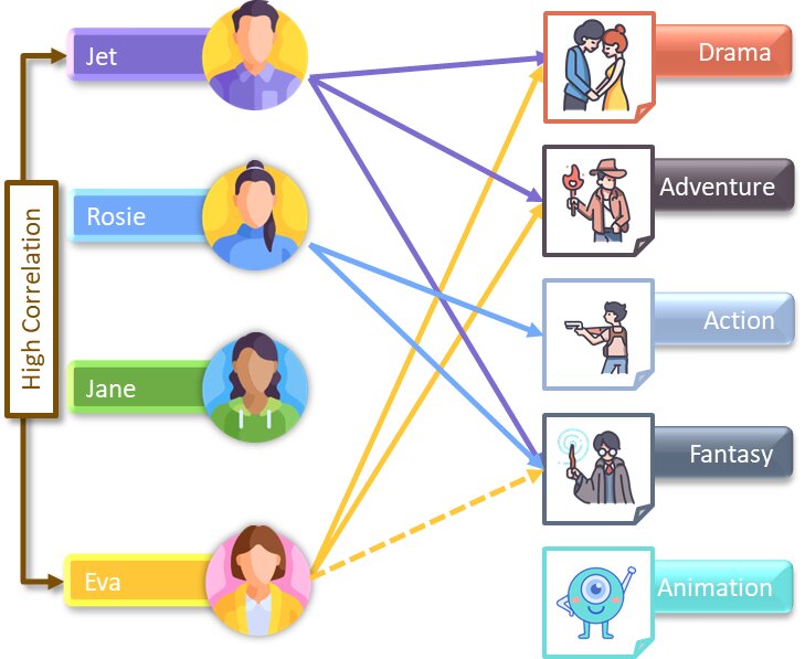
User-Based: Where we try to find similar users based on their item choices and recommend the items. A user-item rating matrix is created at first. Then, we find the correlations between the users and recommend items based on correlation.
Consider the above figure, we can see that:
- Jet likes Drama, Adventure, and Fantasy-based movies.
- Rosie likes Action and Fantasy-based movies.
- Eva likes Drama and Adventure-based movies.
From the above data, we can say that Eva is highly correlated to Jet. Thus, we can recommend her Fantasy movies as well.
Item Based
Where we try to find a similar item based on their user’s choices and recommend the items. A user-user item rating matrix is created at first. Then, we find the correlations between the items and recommend items based on correlation.
Using collaborative filtering becomes stale when either item or user choices differ.
Content-Based Filtering
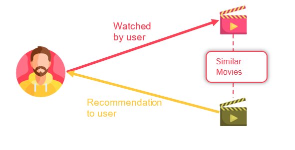
In this type, we will try to find similar items to the user’s selected item. Consider the below figure:
Let’s say Raghu watches a movie X, then in this case the model/method will try to find a similar movie based on its features like genres, actors and directors, etc. For example, if a user likes to watch movies like say Central Intelligence where Dwayne Johnson is the protagonist, the model recommends the movies where Dwayne Johnson is either protagonist or has done some other part in it.
Raghu wants the exact similar type of recommender system where he can input some movie names and related movies are given as recommendations. Let’s see how he will apply machine learning to create a recommendation system.
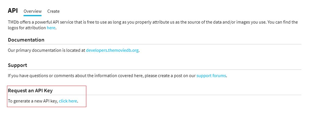
To create the movie recommendation system Raghu has taken data from TMDB API. You can also request an API:
Movie Dataset
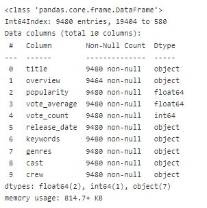
The data gathered by Raghu has the following details:
- Title: Movie Title.
- Overview: Abstract of the Movie.
- Popularity: Movie popularity rating as per TMDB.
- Vote_average: Votes average out of 10.
- Vote_count: Number of votes from the users.
- Release_date: Date of release of the movie.
- Keywords: Keywords for the movie by TMDB in the list.
- Genres: Movie Genres in the list.
- Cast: Cast of the movie on the list.
- Crew: Crew of the movie in the list.
Reading Movies Data:
As Raghu loads the data, let’s see how it looks:
data=pd.read_csv('tmdb.csv.zip',compression='zip',index_col='id') data.head()
Run this demo in Colab – Try it Yourself!

Cleaning Data
As you can see that before applying any machine learning models or even exploring the data we need to clean the data:
Removing Unnamed Column:
The Unnamed Columns are irritating as we cannot delete is normally. To remove this, Raghu gets the list of columns and renames the “Unnamed: 0” column and later removes it:
data.columns=['temp', 'title', 'overview', 'popularity', 'vote_average', 'vote_count', 'release_date', 'keywords', 'genres', 'cast', 'crew'] data.drop('temp',axis=1,inplace=True)
new_types={'title': str, 'overview': str, 'release_date': 'datetime64',} for col in new_types.keys(): data[col]=data[col].astype(new_types[col])
It seems that he has not treated the list columns. The list columns still have some empty values if he changes the type as a list directly he will get the following error:
The error means that it does not support the list datatype as of now. Instead, he creates that column as string type and keeps the values as comma separated:
for col in ['keywords', 'genres', 'cast', 'crew']: for val in ['[',']','\'']: data[col]=data[col].str.replace(val,'') data[col]=data[col].astype(str)
def get_uniques(data,col): ''' data: Dataframe object col: column name with comma separated values --- returns: a list of unique category values in that column ''' out=set([val.strip().lower() for val in ','.join(data[col].unique()).split(',')]) try: out.remove('') except: return list(out) return list(out)
- get_counts(data,col,categories): Returns the counts for the unique items
def get_counts(data, col, categories): ''' data: dataframe object col: name of the column categories: categories present ---- return a dictionary with counts of each category ''' categ = {category: None for category in categories} for category in tqdm(categories): val=0 for index in data.index: if category in data.at[index,col].lower(): val+=1 categ[category]=val return categ
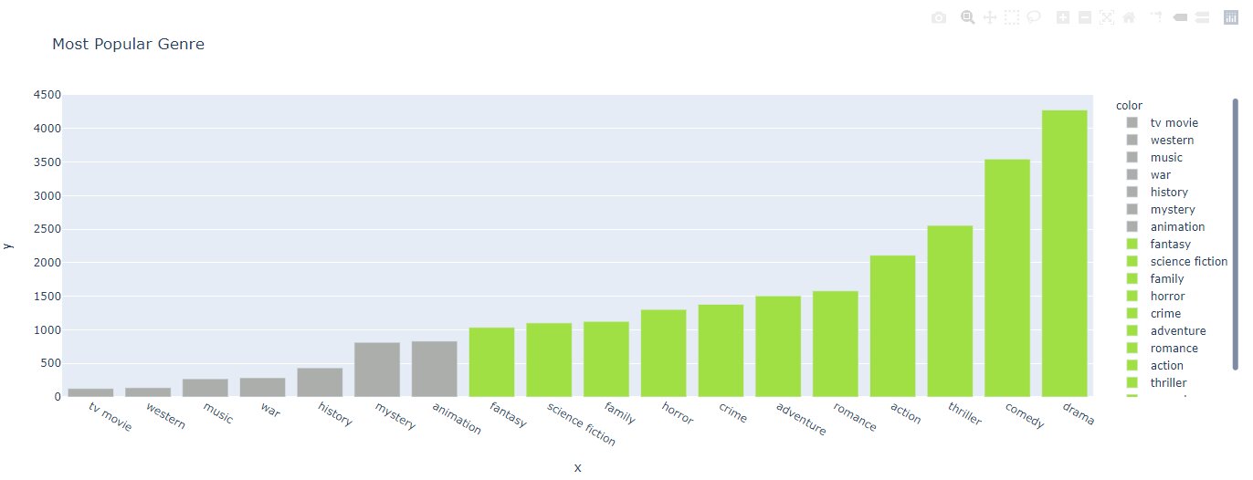
Using the two functions he creates a plotly chart to see most popular genres:
# Get the base counts of for each category and sort them by countsbase_counts = get_counts(data, 'genres', genres)base_counts = pd.DataFrame(index=base_counts.keys(), data=base_counts.values(), columns=['Counts'])base_counts.sort_values(by='Counts', inplace=True)# Plot the chart which shows top genres and separate by color where genre<1000colors=['#abaeab' if i<1000 else '#A0E045' for i in base_counts.Counts]fig = px.bar(x=base_counts.index, y=base_counts['Counts'], title='Most Popular Genre',color_discrete_sequence=colors,color=base_counts.index)fig.show()
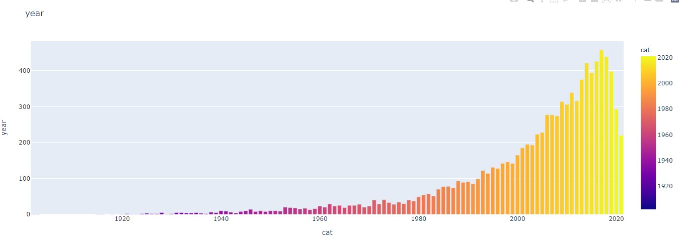
Later, he finds how plots movie release per year:
# Function to plot value counts plotsdef plot_value_counts_bar(data, col): ''' data: Dataframe col: Name of the column to be plotted ---- returns a plotly figure ''' vc = pd.DataFrame(data[col].value_counts()) vc['cat'] = vc.index fig = px.bar(vc, x='cat', y=col, color='cat', title=col) fig.update_layout() return fig data['year']=data.release_date.dt.yearplot_value_counts_bar(data,'year')
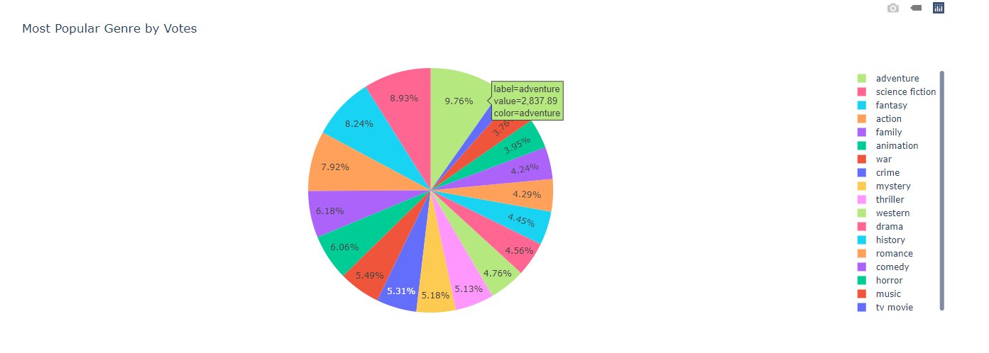
Then, he creates another function to find the ratings by popularity, vote_count, vote_average:
def get_ratings(data, col,ratings_col, categories): ''' data: dataframe object col: name of the column categories: categories present ---- return a dictionary with average ratings of each category ''' categ = {category: None for category in categories} for category in tqdm(categories): val=0 ratings=0 for index in data.index: if category in data.at[index,col].lower(): val+=1 ratings+=data.at[index,ratings_col] categ[category]=round(ratings/val,2) return categbase_counts = get_ratings(data, 'genres','vote_count', genres)base_counts = pd.DataFrame(index=base_counts.keys(), data=base_counts.values(), columns=['Counts'])base_counts.sort_values(by='Counts', inplace=True)fig = px.pie(names=base_counts.index, values=base_counts['Counts'], title='Most Popular Genre by Votes',color=base_counts.index)fig.show()
You can explore more using the above functions like most popular crew, most voted crew.


Building Model
Raghu will be building the model in two ways:
Using CountVectorizer
It converts a collection of text into a matrix of counts with each hit.
Take an example with 3 sentences:
I enjoy Marvel movies.
I like Dwayne.
I like Iron Man.
The count vectorizer will create a matrix where it determines the frequency of each word.
Focusing on the first row, “like” and “enjoy” are besides “I” for 2 and 1 times respectively. Similarly, other rows are calculated.
Raghu, creates the sentences for the CountVectorizer:
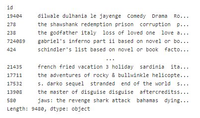
def create_soup(data): # Creating a simple text for countvectorizer to work with att = data['title'].lower() for i in data[1:]: att = att + ' ' + str(i) return att model_data=data.copy()model_data=model_data[['title','keywords','genres','cast','crew']]model_data['soup']=model_data.apply(create_soup,axis=1)
He gets the data in the following way:
Now, he gets the cosine similarity scores:
count = CountVectorizer(stop_words='english')count_matrix = count.fit_transform(model_data['soup'])cosine_sim2 = cosine_similarity(count_matrix)
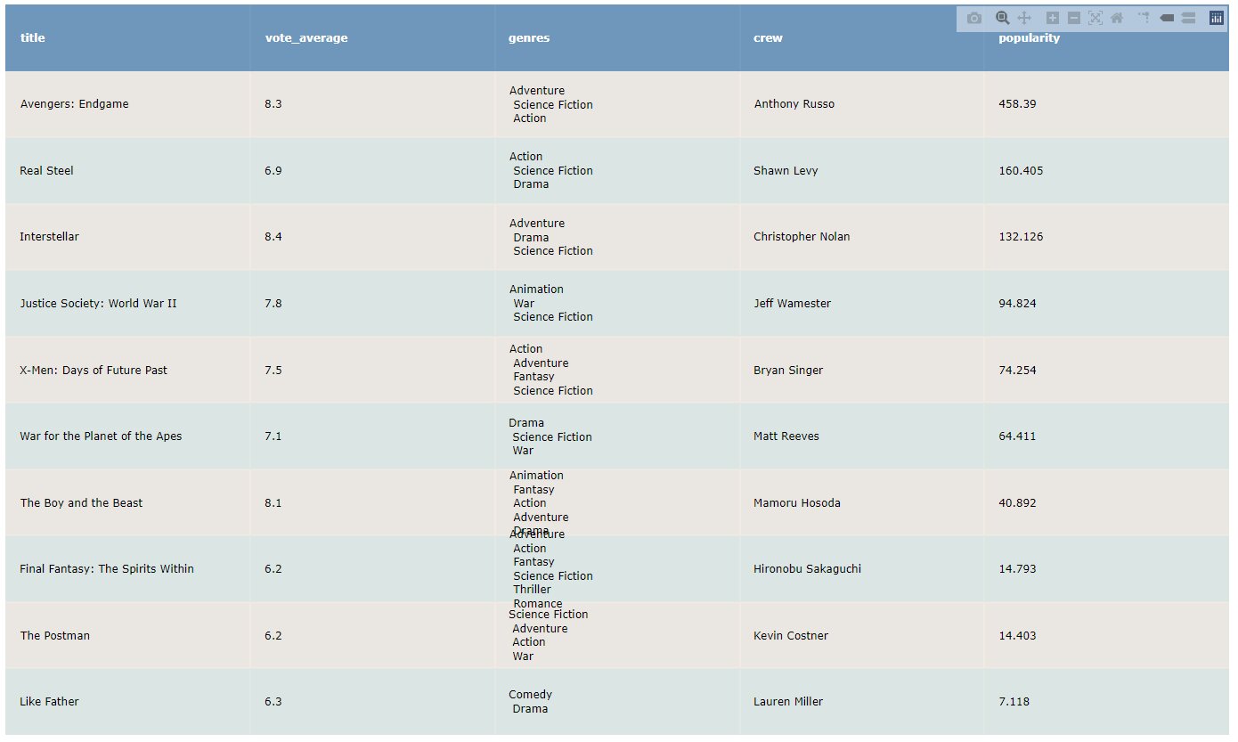
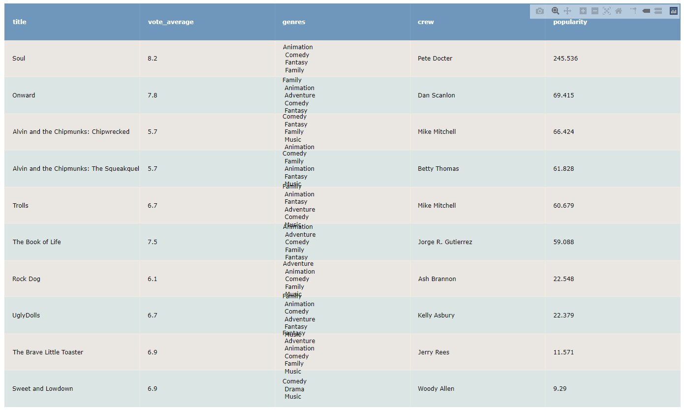
Since we have the cosine similarity scores we can now get the recommendations. The below functions get the top 10 movies sorted by popularity:
def get_recommendations_new(title, data, orig_data, cosine_sim=cosine_sim2): ''' title: movie title data: model_data orig_data: original dataframe cosine_sim: cosine similarity matrix to use. --- returns: Table plot of plotly where top 10 movies by popularity are sorted. ''' indices = pd.Series(data.index, index=data['title']) idx = indices[title] # Get the pairwsie similarity scores of all movies with that movie sim_scores = list(enumerate(cosine_sim[idx])) # Sort the movies based on the similarity scores sim_scores = sorted(sim_scores, key=lambda x: x[1], reverse=True) # Get the scores of the 10 most similar movies sim_scores = sim_scores[1:11] # Get the movie indices movie_indices = [i[0] for i in sim_scores] # Return the top 10 most similar movies out=orig_data[[ 'title', 'vote_average', 'genres', 'crew', 'popularity' ]].iloc[movie_indices] out.genres = out.genres.str.replace(',', '<br>') out.crew = out.crew.str.replace(',', '<br>') final=out.sort_values(by='popularity',ascending=False) colorscale = [[0, '#477BA8'], [.5, '#ece4db'], [1, '#d8e2dc']] fig = ff.create_table(final, colorscale=colorscale, height_constant=70) return fig
nn_data=data.copy()def fill_genre(value,col,categories=genres): if col in value.lower() : return 1 else: return 0# Create genre columnsfor col in genres: nn_data[col]=Nonefor index in tqdm(nn_data.index): for col in genres: nn_data.at[index,col]=fill_genre(nn_data.at[index,'genres'],col)for col in genres: nn_data[col]=nn_data.genres.apply(fill_genre,args=(col,))nn_data.drop(['overview','release_date','genres','title'],axis=1,inplace=True)for col in ['keywords','cast','crew']: nn_data[col]=LabelEncoder().fit_transform(nn_data[col])
Traning the model:
model_knn = NearestNeighbors(metric='cosine', algorithm='auto', n_neighbors=20, n_jobs=-1)model_knn.fit(nn_data)
Now, Let’s test our model:
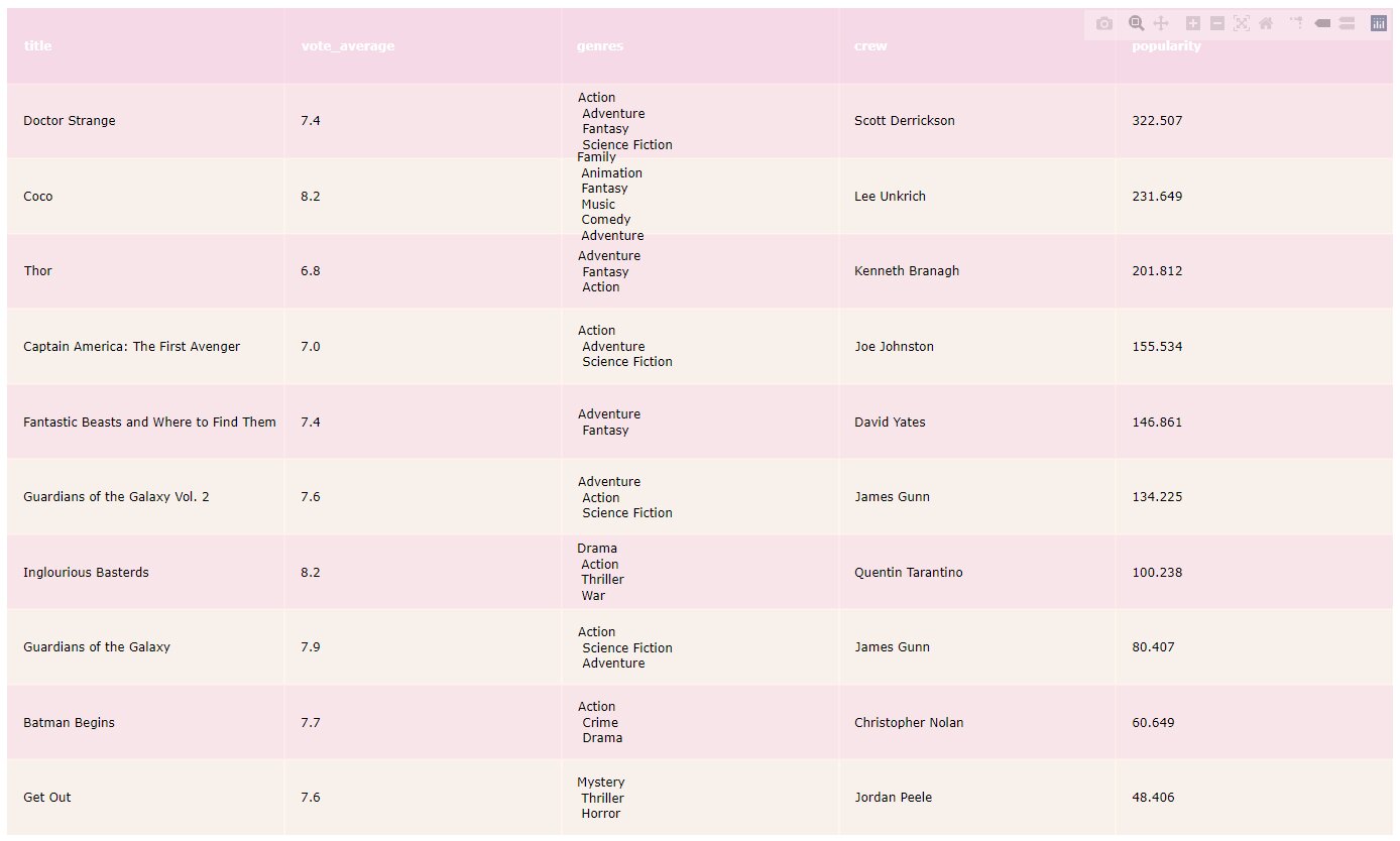
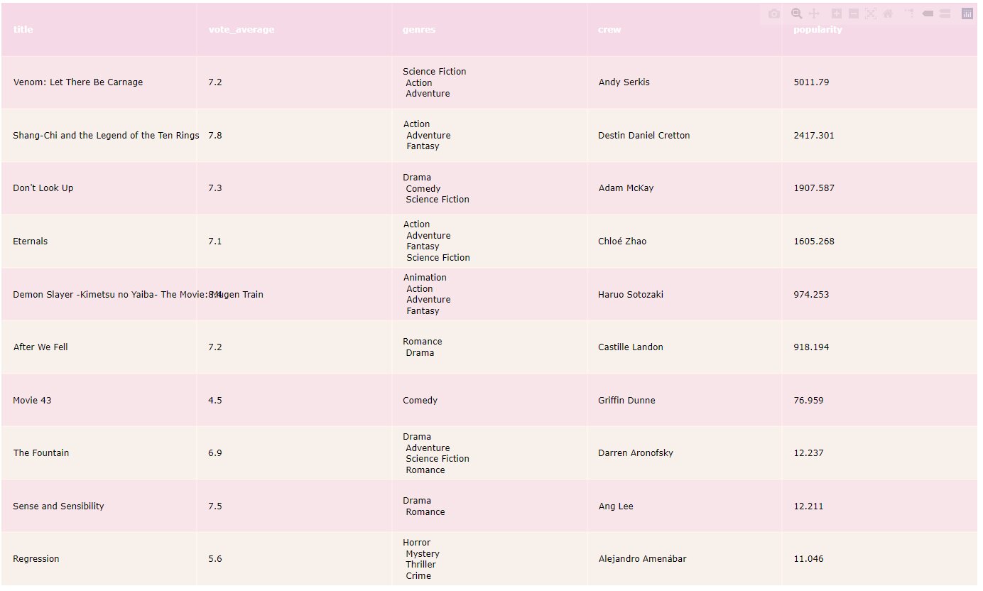
# Create a function to recommend top 10 moviesdef recommend_movies(movie,nn_data,orig_data): orig_data.reset_index(inplace=True) nn_data.reset_index(inplace=True,drop=True) movie_index=nn_data[orig_data.title==movie].index distances, indices = model_knn.kneighbors(np.array(nn_data.iloc[movie_index]).reshape( 1, -1),n_neighbors=10) out=orig_data[[ 'title', 'vote_average', 'genres', 'crew', 'popularity' ]].iloc[indices[0]] out.genres = out.genres.str.replace(',', '<br>') out.crew = out.crew.str.replace(',', '<br>') final=out.sort_values(by='popularity',ascending=False) colorscale = [[0, '#fad2e1'], [.5, '#fde2e4'], [1, '#fff1e6']] fig = ff.create_table(final, colorscale=colorscale, height_constant=70) return fig
Let’s check for the movie “Thor”:
Let’s try for “Eternals”:
Run this demo in Colab – Try it Yourself!

This is a collection of insightful articles from domain experts in the fields of Cloud Computing, DevOps, AWS, Data Science, Machine Learning, AI, and Natural Language Processing. The range of topics caters to upski... Read Full Bio


