Naïve Bayes Algorithm in Machine Learning
When working with Machine Learning problems that deal with labeled training datasets, the algorithms are categorized as either classification or regression. When you go a little deeper, one of the most fundamental algorithms you will encounter is Naïve Bayes Algorithm.
Let me paint a picture for you. Your new year resolution is to keep your health in check and so you decide to develop a running habit. Now, let’s say you want to predict if you will go for a run or not based on the weather conditions outside.
So, this becomes a classification problem.
Naïve Bayes is a simple classification algorithm that can help you with your model.
In this blog we will cover the following sections:
- Quick Introduction to Bayes Theorem
- Stepwise Bayes Theorem
- The Naïve Bayes Algorithm
- Industrial Applications of Naïve Bayes
- Types of Naïve Bayes Classifiers
- Advantages of Naïve Bayes
- Limitations of Naïve Bayes
- Naïve Bayes Demo Using Python
Quick Introduction to Bayes Theorem
The Bayes in Naïve Bayes comes from Bayes’ Theorem. If you paid attention to probability and statistics in your maths class, there’s little chance you haven’t already heard of Bayes’ theorem. Let’s recall it:
Bayes’ Theorem describes the probability of an event based on prior knowledge of the conditions that might be related to the event.
This equation is derived from the formula of conditional probability given below:
Let’s take a silly little example – Say the likelihood of a person having Arthritis if they are over 65 years of age is 49%.
Check the above stats at: Centre for Disease Control and Prevention
Now, let’s assume the following:
- Class Prior: The probability of a person stepping in the clinic being >65-year-old is 20%
- Predictor Prior: The probability of a person stepping into the clinic having Arthritis is 35%
What is the probability that a person is >65 years given that he has Arthritis? This is Let’s calculate this with the help of Bayes’ theorem!
In fact, Bayes’ Theorem is nothing but an alternate way of calculating the conditional probability of an event. When the reverse conditional probability is easier to calculate than the joint probability, Bayes’ Theorem is used.
You can use Bayes’ theorem to build a learner ML model, from an existing set of attributes, that predicts the probability of the response variable belonging to some class, given a new set of attributes.
Consider the previous equation again. Now, assume that event A is the response variable and event B is the input attribute. So according to the equation,
- P(A) or Class Prior is the prior probability of the response variable
- P(B) or Predictor Prior is the evidence or the probability of training data
- P(A|B) or Posterior Probability is the conditional probability of the response variable being of a particular value given the input attributes
- P(B|A) or Likelihood is basically the reverse of the posterior probability or the likelihood of training data
Best-suited Machine Learning courses for you
Learn Machine Learning with these high-rated online courses
Stepwise Bayes Theorem
Let’s come back to the problem at hand. Looks like you’re very serious with your resolution this time given that you have been keeping track of the weather outside for the past two weeks:
Step 1 – Collect raw data
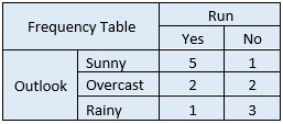
Next, you need to create a frequency table for each attribute of your dataset.
Step 2 – Convert data to a frequency table(s)
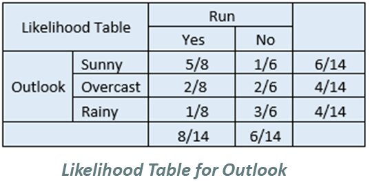
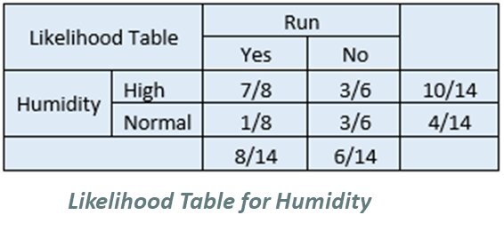
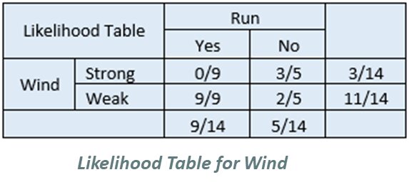
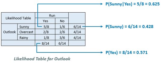
Then, for each frequency table, you will create a likelihood table.
Step 3 – Calculate prior probability and evidence
Step 4 – Apply probabilities to Bayes’ Theorem equation
Let’s say you want to focus on the likelihood that you go for a run given that it’s sunny outside.
P(Yes|Sunny) = P(Sunny|Yes) * P(Yes) / P(Sunny) = 0.625 * 0.571 / 0.428 = 0.834
The Naïve Bayes Algorithm
Naïve Bayes assumes conditional independence over the training dataset. The classifier separates data into different classes according to the Bayes’ Theorem. But assumes that the relationship between all input features in a class is independent. Hence, the model is called naïve.
This helps in simplifying the calculations by dropping the denominator from the formula while assuming independence:
Let’s understand this through our running resolution example:
Say you want to predict if on the coming Wednesday, given the following weather conditions, should you go for a run or sleep in:
Outlook: Rainy
Humidity: Normal
Wind: Weak
Run: ?
Likelihood of ‘Yes’ on Wednesday:
P(Outlook = Rainy|Yes) * P(Humidity = Normal|Yes) * P(Wind = Weak|Yes) * P(Yes)
= 1/8 * 1/8 * 9/9 * 8/14 = 0.0089
Likelihood of ‘No’ on Wednesday:
P(Outlook = Rainy|No) * P(Humidity = Normal|No) * P(Wind = Weak|No) * P(No)
= 3/6 * 3/6 * 2/5 * 6/14 = 0.0428
Now, to determine the probability of going for a run on Wednesday, you just need to divide P(Yes) with the sum of the likelihoods of Yes and No.
P(Yes) = 0.0089 / (0.0089 + 0.0428) = 0.172
Similarly, P(No) = 0.0428 / (0.0089 + 0.0428) = 0.827
According to your model, it looks like there’s an almost 83% probability that you’re going to stay under the covers next Wednesday!
This was just a fun example. Although Naïve Bayes IS used for weather predictions, for advanced machine learning problems, the complexity of the Bayesian classifier needs to be reduced for it to be practical. This is where the naïve in Naïve Bayes comes in.
Industrial Applications of Naïve Bayes
- Text Classification: Naïve Bayes algorithm is almost always used as a classifier and is an excellent choice for spam filtering of your emails or news categorization on your smartphone.
- Recommendation Systems: Naïve Bayes is used with collaborative filtering to build recommendation systems for you. The ‘Because you watched ____’ section on Netflix is exactly that.
Sentiment Analysis: Naïve Bayes is an effective algorithm for the identification of positive or negative sentiments of a target group (customers, audience, etc.). Think of feedback forms and IMDb reviews.
Types of Naïve Bayes Classifiers
Bernoulli Naïve Bayes
- Predictors are Boolean variables
- Used when data is as per multivariate Bernoulli distribution
- Popular for discrete features
Multinomial Naïve Bayes
- Uses frequency of present words as features
- Commonly used for document classification problems
- Popular for discrete features as well
Gaussian Naïve Bayes
- Used when data is as per the Gaussian distribution
- Predictors are continuous variables
Advantages of Naïve Bayes
- Easy to work with when using binary or categorical input values.
- Require a small number of training data for estimating the parameters necessary for classification.
- Handles both continuous and discrete data.
- Fast and reliable for making real-time predictions.
Limitations of Naïve Bayes
- Assumes that all the features are independent, which is highly unlikely in practical scenarios.
- Unsuitable for numerical data.
- The number of features must be equal to the number of attributes in the data for the algorithm to make correct predictions.
- Encounters ‘Zero Frequency’ problem: If a categorical variable has a category in the test dataset that wasn’t included in the training dataset, the model will assign it a 0 probability and will be unable to make a prediction. This problem can be resolved using smoothing techniques which are out of the scope of this article.
- Computationally expensive when used to classify a large number of items.
Naïve Bayes Demo Using Python
Now that we have learned what Naïve Bayes is, let’s learn how to apply this algorithm in Python using the scikit-learn library using the following steps –
- Analyze the given dataset
- Check the distribution of the target variable
- Encode target variable
- Convert the categorical features to dummy data
- Split our data into train and test data
- Assume a normal distribution
- Calculate the accuracy scores of models
Let’s say you have data on a company’s employees, and you wish to classify employees with salaries greater than 50K.
Step 1 – Let’s start with analyzing the given dataset
#Read the datatsetincome_data=pd.read_csv('income_evaluation.csv') #Display the first five rowsincome_data.head()
#Number of rows and columnsincome_data.shape
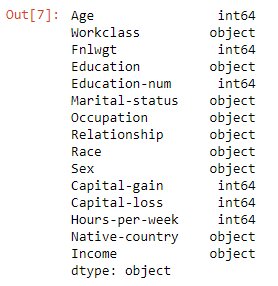
#Check the data typesincome_data.dtypes
Run this demo – Try it yourself!
Click the below image to run this demo.

We will encode the categorical features later.
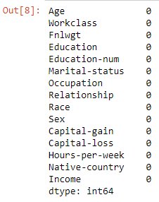
#Test null valuesincome_data.isnull().sum()
#Test NA valuesincome_data.isna().sum()
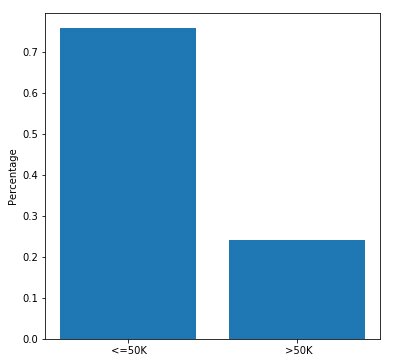
2 – Now, we will check the distribution of our target variable, ‘Income’
Target_ratio=income_data['Income'].value_counts()/len(income_data)print(Target_ratio)
#Check for data unbalanceplt.figure(figsize = (6,6))plt.bar(Target_ratio.index,Target_ratio)plt.ylabel('Percentage')plt.show()
The dataset has around 24% of entries where income is >50K.
3 – Let’s now encode our target variable
lb=LabelEncoder()income_data.Income=lb.fit_transform(income_data.Income) lb.classes_
We see that there are two classes in the dataset.
4 – Now we convert the categorical features to dummy data
cat_features=income_data.columns[income_data.dtypes=='O']print(*cat_features,sep=' | ') # * is wildcard to print a list, where parameter sep is used to define a separator.
new_data = pd.get_dummies(income_data, columns = cat_features)new_data.head()
5 – Let’s split our data into train and test data
X=new_datay=new_data.Income X_train, X_test, y_train, y_test=train_test_split(X,y,random_state=0,test_size=0.3)
6 –Assuming a normal distribution
Now comes the interesting part, we will fit our data into Gaussian and Bernoulli Naïve Bayes models:
Training Gaussian Naive Bayes
gaussian_nb=GaussianNB()gaussian_nb.fit(X_train,y_train)
Training Bernoulli Naive Bayes
bernoulli_nb=BernoulliNB() bernoulli_nb.fit(X_train,y_train
Step 7 – Let’s calculate the accuracy scores of our models
Gaussian Naive Bayes Accuracy Score
pred=gaussian_nb.predict(X_test)acc_gnb=accuracy_score(y_test,pred)print('Accuracy Score: ',acc_gnb)
Bernoulli Naive Bayes Accuracy Score
pred=bernoulli_nb.predict(X_test)acc_bnb=accuracy_score(y_test,pred)print('Accuracy Score: ',acc_bnb)
Let’s plot it, shall we?
Looks like Bernoulli clearly has better accuracy than the Gaussian model in this case.
Endnotes
Despite being over-simplified to the point of being called naïve, the Bayesian classifier has found its use in many real-world applications. Machine Learning is an increasingly growing domain that has been adopted by various sectors in the IT industry and hugely impacts big businesses worldwide.
This is a collection of insightful articles from domain experts in the fields of Cloud Computing, DevOps, AWS, Data Science, Machine Learning, AI, and Natural Language Processing. The range of topics caters to upski... Read Full Bio


