4 Ways to TRANSPOSE in Excel – Shiksha Online

Learn how to transpose data in Excel and quickly change the orientation of columns and rows in a spreadsheet.

TRANSPOSE function is categorized under Excel Lookup and Reference functions. It flips the direction of a given array or data range. TRANSPOSE in Excel changes or rotates data from the horizontal array to the vertical array. You can transpose data using different ways, including the TRANSPOSE function, Paste Special method, and direct references method. This article will show you how to TRANSPOSE data using the above-mentioned methods.

Content

• Using TRANSPOSE Function
• Paste Special Transpose
• Transposition Of Data With Direct References
• Transpose Data Using Power Query 
• Points to remember

1. Using TRANSPOSE Function

You can change the orientation of an array using the TRANSPOSE function from vertical to horizontal or vice versa. An array formula requires you to enter the function in a range with the same number of rows and columns as the source.

The syntax of the transpose function is:

=Transpose(array)

The following sample spreadsheet will transpose the array with employee names, departments, countries of origin, and payouts.

First, find out how many rows and columns are in your original array. After that, select the exact number of cells as the original range, but in the other direction.

For example, we have five rows and three columns, so we must select three rows and five columns of cells for the transposed data. 

In our case, we have five rows and four columns, so you need to select four rows and five columns.

Select a blank range of cells and enter the formula: 

=TRANSPOSE(A3:D12)

Do not press the ‘Enter’ key. At this stage, your spreadsheet will look like this –

Now, press ‘Ctrl + Shift + Enter’, this will transpose the data. Remember, it’s a mandatory step.

An array formula must permanently be terminated by pressing CTRL + SHIFT + ENTER. This combination places a set of brackets around the formula in the formula bar. This ensures that the result is treated as an array of data and not a single cell value.

Note – While using the TRANSPOSE formula, count and select the given number of columns/rows only. You won’t be able to change that further (check below).

Excel’s TRANSPOSE function only copies data, not the formatting of the original data. Excel does not copy the original header formatting. It is a dynamic function. When its value changes in the original data, it reflects in the transposed data.

Explore MS Excel Courses

2. Paste Special Transpose

You can use the Paste Special option in Excel to paste the transposed data. 

Create a table adjacent to your existing array and copy your data.

Select the new table array and go to Paste ⇒ Paste Special.

A window with different options to format your content will pop up before pasting it. Locate Transpose and check that option.

Your table data has now been transposed on the adjacent table array.

3. Transposition of Data with Direct References

In our third Excel data transposition method, we will use direct references. This method allows us to find and replace a reference with the data we want to display.

Click on an empty cell, type a reference, and then the location of the first cell we want to transpose. In this circumstance, I will use raA2.

Below raA2, write raB2.

Highlight both cells and drag the highlighted area out by clicking and dragging the green box at the bottom right of the selection.

Press Ctrl + H on your keyboard to open the “Find and Replace” menu. Go to Replace option and in the “Find what” field, type the selected prefix, “ra” (without quotes), and then “=” (without quotes) in the “Replace with” field. Now click “Replace all.”

You will see that the number of selected cells has the required information.

4. Transpose Data Using Power Query 

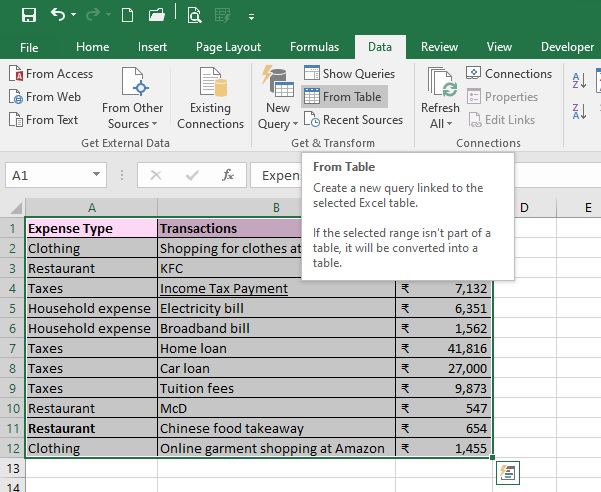
Select the range of data that you want to transpose. 

Go to the Data tab → Click on From Table. 

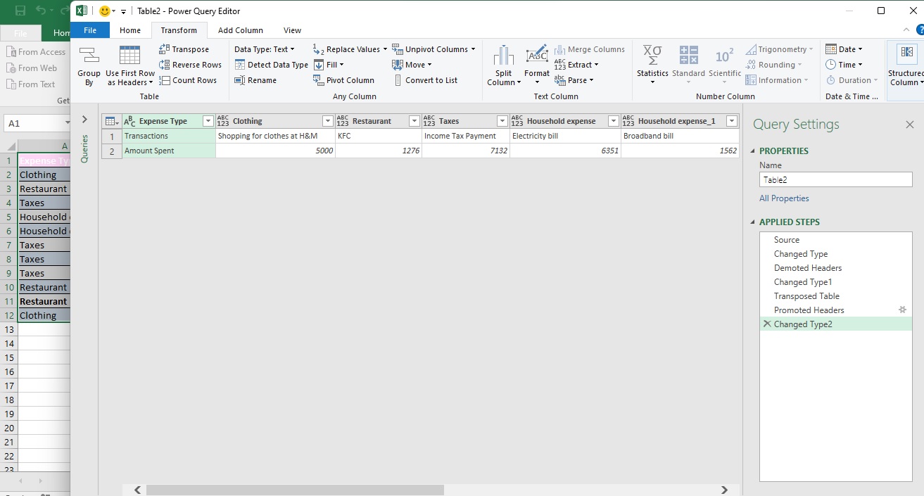
Power Query Editor will open. 

On the editor, go to –

Transform → Table → Use First Row as Headers → Use Headers as First Row. 

By selecting this option, all the headers move to the first row. 

Click Transpose to transpose the data.

Select – ‘Use First Row as Headers.’ to keep the first row of transposed data as a header. 

Click File tab → Close & Load. 

The transposed data will now be loaded onto the spreadsheet.

Points to remember

• TRANSPOSE in Excel changes columns to rows and vice versa.
• Enter the TRANSPOSE function as an array formula with the same number of cells as the array 
• Press Ctrl + Shift + Enter to apply the formula, not just Ctrl.
• The new array must occupy the exact count of rows as the source array has columns and vice versa.

Conclusion

To transpose data manually is a time-consuming task. Using Transpose in Excel will help you in data analysis and management. We hope this article helped you understand Transpose in Excel and how to transpose data using different methods.

Top Trending Articles in MS Excel:

Most Useful Excel Formulas | Min Max Functions in Excel | Average Functions in Excel | Introduction to MS Excel | Financial Modelling in Excel | MS Excel interview questions | Sum Function in Excel | Trim Function in Excel | Pivot Table in Excel | Percentage in Excel | Vlookup in Excel | Median Function in Excel | Types of Charts in Excel | Count Function in Excel | MS Excel Vs. Google Sheet | Remove Duplicates in Excel | Create Graph in ExcelConclusion