Tutorial – VLOOKUP in Excel – Shiksha Online

VLOOKUP, or vertical lookup, is one of Excel’s most commonly used functions for data analysis. This function belongs to the Search and Reference group, which has other search functions in Excel. In this tutorial, we will cover VLOOKUP in Excel and how it works through examples.

• Definition: What is VLOOKUP?
• VLOOKUP Formula
• How to Use VLOOKUP in Excel?
• Conclusion

Must Read – What is MS Excel?

Definition: What is VLOOKUP?

The VLOOKUP function gets its name because it does vertical lookups. The letter “V” in the VLOOKUP function suggests that the function will perform a vertical search, a search on a column of data. The VLOOKUP function is undoubtedly the most used.

The VLOOKUP function looks for a value vertically and returns a value from a different column in the same row as the value found.

Explore MS Excel Courses

By telling the function the value we want to find, it will analyze each cell of the search column from top to bottom and stop when the first match is found.

Once the searched value is found, the function will be able to return the value of any column of the data as long as it is in the same row as the value found. Although the function’s operation is straightforward, it is common for Excel users to encounter some difficulty when using it. We have tried to explain VLOOKUP in Excel through examples.

Do you want to learn Excel? Become an expert with our MS Excel Courses.

VLOOKUP Formula

=VLOOKUP(lookup_value, table_array, col_index_num, [range_lookup])

We have four arguments in VLOOKUP.

1. Lookup_value (required): In the first argument, we must indicate the value we are looking for. This value will be searched for, from top to bottom, in the first column of the search range. We can enter the value directly, numerically or text string, or place a reference to a cell containing the value sought. The VLOOKUP function will not be case-sensitive.
2. Table_array (required): The second argument is a cell reference that defines the range where the search will be performed. The VLOOKUP function will always search the first column of that range, and the rest of the column numbers can be returned.

3. Col_index_num (required): The third argument is a numeric value that allows us to indicate the column that we want as a result of finding a match. The columns are not the Excel sheet but the columns of the range stated in the second argument ( Array_search_in ), where the first column will be assigned the number 1.

4. Range_lookup (optional): The fourth and last argument to the VLOOKUP function helps tell the function what type of search we want to perform, whether exact or approximate. 

FALSE – Exact match

TRUE – Approximate search

If we omit this argument, the VLOOKUP function will assume a TRUE value, thus giving a true approximate match.

How to Use VLOOKUP in Excel?

Let’s understand how VLOOKUP works using these examples. We have covered the following –

1. Example 1 – Finding Numeric Values
2. Example 2 – Finding Text Strings

1. Finding Numeric Values

Problem Statement: Find the amount paid by an individual

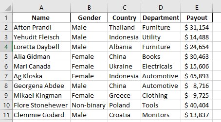
Dataset Attributes: Title, Name, Gender, Country, and Amount Paid.

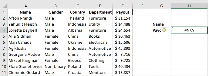
Step 1: Mark two cells with Name and Amount Paid. To start applying the VLOOKUP formula, we will pick a cell and type =VLOOKUP(

Step 2: Enter the value you want to search for. Since we want the value to appear in the above cell, we will mention B14 after the opening parenthesis. =VLOOKUP (H3,

Here H3 is the cell where we want the final result to appear (lookup_value)

Step 3: Enter the range of cells where this value might appear. In this case, the value (Name and Amount Paid) lies in the range (A:E).

=VLOOKUP(H3,A:E

We have selected the entire columns from A to E. The formula will still fetch the results if we add data in these columns.

Step 4: Enter the column index number with the data you seek. In the above range of data, the column of amount paid is in E, whose location is 5th. Hence the lookup values are: (H3,A:E,5

Step 5: Enter the range lookup value, either TRUE or FALSE.

TRUE finds partial matches, while FALSE searches for exact matches.

The final formula is =VLOOKUP(H3,A:E,5,FALSE)

Once you press Enter, you will get N/A in the targeted cell once you press Enter, but there is no need to worry. 

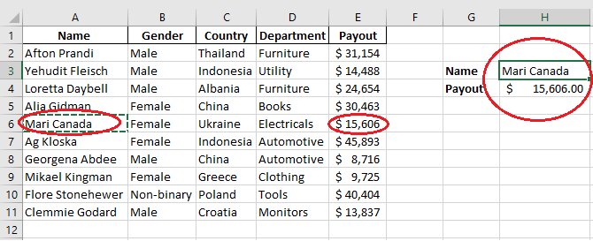
Step 6: Add a name from the Name column and paste it into H2; you will get the amount paid by the selected individual.

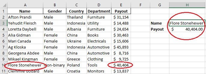
Similarly, without changing the formula, you can paste any other value (Name) from the B column of the table in H3 to get the desired result.

2. Finding Text Strings using VLOOKUP

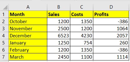
Problem Statement: Search for profits in a particular month

Dataset Attributes: Month, Sales, Costs, and Profits.

Apart from searching for numeric values, VLOOKUP also searches for text strings. This text string can be found against a numeric value in the below dataset.

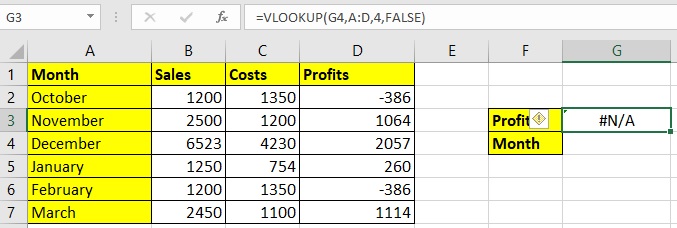
Step 1: Write =VLOOKUP( in G3. We want the text string to appear against the given numeric value in G4. Mention both the requirements here, Profits and Months in G3 and G4.

 

Step 2: Now write the table_array, which is A:D.

Step 3: Mention the col_index_num, which is 4 here.

Step 4: Mention the range_lookup. Choose TRUE if you want the approximate match or FALSE if you want an exact match.

The final formula is =VLOOKUP(G4,A:D,4,FALSE)

Step 5: Press Enter. You will get N/A as a result.

However, since your cell has the correct formula, you can use the numeric value from the D column to check the Text string against it.

Conclusion

VLOOKUP is an extremely popular MS excel function; you must have a good command of it if you are learning Excel. You can have a good command of it if you practice with datasets. I will cover the HLOOKUP function in the upcoming Excel tutorial with examples.

Keep learning!

Read More in Excel

MIS Reports in Excel | Excel Interview Questions | Basic Excel Formulas | Difference Between Formula and Function in Excel | Average Function in Excel | Introduction to MS Excel | HLOOKUP in Excel | ROW and COLUMN in Excel | Financial Modelling in Excel | Percentage In Excel | Remove Duplicates In Excel | Merge Cells in Excel | MIN and MAX Functions in Excel | Combine Text Strings in Excel | Import Data from PDF to Excel | Pivot Table In Excel | How To Enable Macros In Excel | How to Import Text Files to Excel | TRIM Function in Excel