Feature selection Techniques|python code

Feature selection is a method of filtering out the important features as all the features present in the dataset are not equally important. There are some features that have no effect on the output. So we can skip them. As our motive is to reduce the data before feeding it to the training model. So feature selection is performed before training machine learning models. The models with less number of features have higher explainability, it is easier to implement machine learning models with reduced features. Feature selection removes data redundancy. Feature selection is performed after feature engineering.

This blog is mainly for those who want to learn feature selection implementation. But if you are not aware of the basics of feature selection or are a beginner then you can go and see my previous blog, where I covered feature selection techniques also and their differences. You don’t have to learn all the techniques. I will be covering the main important techniques for feature selection with their implementation. All these techniques are trying to find the common thing i.e dependency of independent features and dependent features. The more the dependency the more important will be the feature. So accordingly we will be selecting the features based on the output we receive on implementing these techniques.

I will recommend you to read the blog on feature selection techniques for understanding the working of these techniques before moving to its implementation.

Feature selection python

Now comes the fun part!!!

We will see the practical implementation of this concept. I have taken a data set wine.csv.This dataset was taken purposely. This dataset contains no missing, NaN values and categorical features. This simply means the data preprocessing step is not much required.

Problem statement: Chemical analysis of wines grown in the same region and to determine the quantities of 13 constituents found in each of the three types of wines.

Pearson Correlation

Importing libraries and reading dataset

import pandas as pd
import numpy as np
import seaborn as sns
import matplotlib.pyplot as plt
%matplotlib inline
 
df = pd.read_csv("wine.csv")
df 

If you are new to machine learning coding let me tell you that you have to load the dataset first before executing the above code.

Independent and dependent variables

y = data['Class']
 #Load X Variables into a Pandas Dataframe with columns 
X = data.drop(['Class'], axis = 1)
 y is dependent variable and X is independent variable.

Split the data into train and test data

from sklearn.model_selection import train_test_split
X_train, X_test, y_train, y_test = train_test_split(X, y,random_state=100 test_size=0.3)    

Using Pearson Correlation

cor = X_train.corr()
plt.figure(figsize=(12,10))
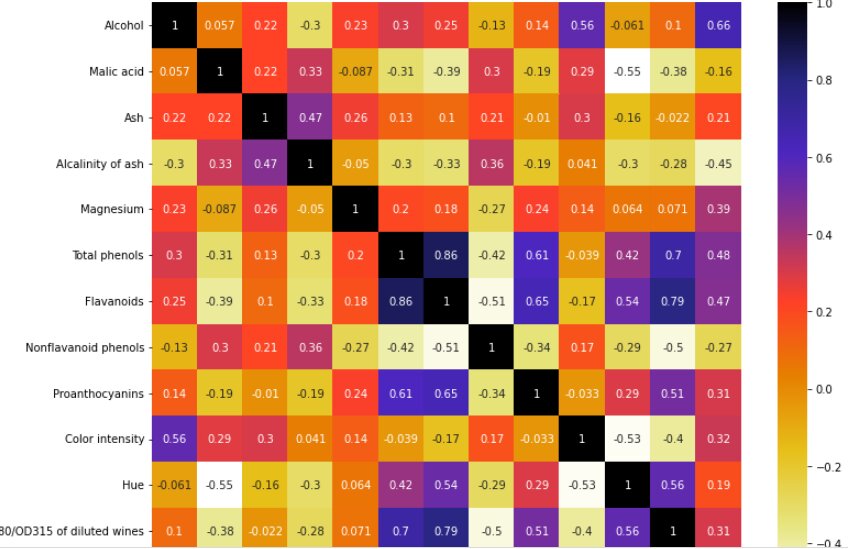
sns.heatmap(cor, cmap=plt.cm.CMRmap_r,annot=True)
plt.show()  
   

This heatmap shows the correlation of all the features of the dataset.

Finding the correlated features

def correlation(dataset, threshold):
    col_corr = set()  
    corr_matrix = dataset.corr()
    for i in range(len(corr_matrix.columns)):
        for j in range(i):
            if abs(corr_matrix.iloc[i, j]) > threshold: colname = corr_matrix.columns[i]                  
col_corr.add(colname)
return col_corr      

With the help of this function, we can select highly correlated features. The purpose is to select the correlated features and then remove them. If you note then we have written abs means absolute, because we will get a negative correlation also which will convert into a positive.

Now the very important question arises here Can we do the same for test data also. The answer is NO. Why? In order to avoid overfitting. Here we have to set the threshold value for correlation also.

Getting correlated features

corr_features = correlation(X_train, 0.7)
Corr_features
Output:
{'Flavanoids', 'OD280/OD315 of diluted wines'}
     

Like here we set threshold=0.7 which means the features which are 70% or more correlated will be returned in the output. You can set any value of the threshold. Most people set it to be 0.85.

Removing correlated features

X_train.drop(corr_features,axis=1)
X_test.drop(corr_features,axis=1)
X_train     

Chi-square

Perform chi2 test

from sklearn.feature_selection import chi2
Calculating Fscore and p value
f_p_values=chi2(X_train,y_train)
F_p_values
 
output:
(array([4.22853570e+00, 2.37537819e+01, 6.85971917e-01, 2.51905256e+01,
        2.98617377e+01, 1.30515334e+01, 5.15232527e+01, 1.51782774e+00,
        8.08914504e+00, 8.94909592e+01, 4.33089278e+00, 2.02933327e+01,
        1.33574764e+04]),
 array([1.20721644e-01, 6.94915188e-06, 7.09648176e-01, 3.38802707e-06,
        3.27797807e-07, 1.46519534e-03, 6.48437052e-12, 4.68174650e-01,
        1.75171913e-02, 3.69219925e-20, 1.14698723e-01, 3.92065660e-05,
        0.00000000e+00]))      

Chi-square is used to find F-score and p-values for all features. So in this case the first array is for F score and the second array is for p- values. Now, what is the importance of these two values? And the more the value of the F score the more important the feature is and the lesser the value of the p-value the more important will be the feature.

Representing in list form

import pandas as pd
p_values=pd.Series(f_p_values[1])
p_values.index=X_train.columns
P_values        

Sorting values in ascending order

p_values.sort_index(ascending=False)
 
Output:
Total phenols 1.465195e-03
Proline 0.000000e+00
Proanthocyanins 1.751719e-02
OD280/OD315 of diluted wines 3.920657e-05
Nonflavanoid phenols 4.681746e-01
Malic acid 6.949152e-06
Magnesium 3.277978e-07
Hue 1.146987e-01
Flavanoids 6.484371e-12
Color intensity 3.692199e-20
Ash 7.096482e-01
Alcohol 1.207216e-01
Alcalinity of ash 3.388027e-06
dtype: float64        

Observation

The total phenols Column is the most important column when compared to the output feature.

Now let’s learn the third very important technique i.e feature selection by using mutual information gain.

Mutual information gain

Importing mutual information gain

from sklearn.feature_selection import mutual_info_classif
# determine the mutual information
mutual_info = mutual_info_classif(X_train, y_train)
mutual_info
 
Output:
array([0.45810181, 0.26490518, 0.05332173, 0.2187717 , 0.25110079,
       0.41649437, 0.68865959, 0.08089527, 0.29778143, 0.5377321 ,
       0.47179421, 0.48180695, 0.53742616])
 

mutual_info_classif is a library that is present in feature_selection. It is the property of mutual information gain that the value you will get will never be negative. The higher the value the more important that feature will be or you can say that the dependency of that independent feature will be more on the dependent feature.

Representing in list form

mutual_info = pd.Series(mutual_info)
mutual_info.index = X_train.columns
mutual_info.sort_values(ascending=False)
Output:
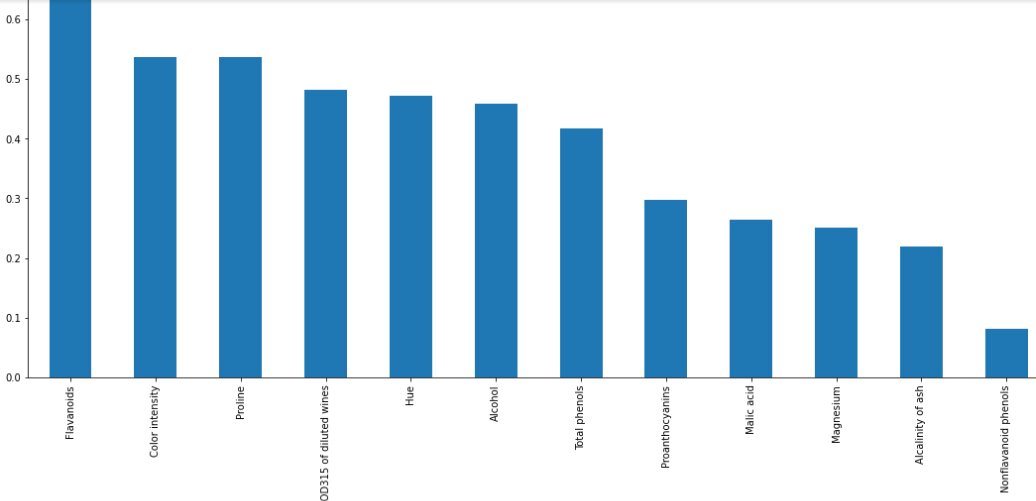
Flavanoids 0.688660
Color intensity 0.537732
Proline 0.537426
OD280/OD315 of diluted wines 0.481807
Hue 0.471794
Alcohol 0.458102
Total phenols 0.416494
Proanthocyanins 0.297781
Malic acid 0.264905
Magnesium 0.251101
Alcalinity of ash 0.218772
Nonflavanoid phenols 0.080895
Ash 0.053322
dtype: float64

Plotting the graph

plot the ordered mutual_info values per feature

mutual_info.sort_values(ascending=False).plot.bar(figsize=(20, 8)

Selecting best 5 features

from sklearn.feature_selection import SelectKBest
#No we Will select the top 5 important features
sel_five_cols = SelectKBest(mutual_info_classif, k=5)
sel_five_cols.fit(X_train, y_train)
X_train.columns[sel_five_cols.get_support()]
Output:
Index(['Flavanoids', 'Color intensity', 'Hue', 'OD280/OD315 of diluted wines','Proline'],dtype='object')
   

Assignment

I suggest you download this dataset and try these techniques first and then try it on some big datasets. You will get the same dataset on Kaggle and Github. You can try the Pima Indians Diabetes dataset also for your practice.

Endnotes

We can judge features’ importance by ourselves also, based on our knowledge and experience. This blog included the code for the different feature selection techniques.

If this blog helped you in any way then please share it with other data science aspirants also. If you are interested in going into the data science field then you find different study material on this page.

Share knowledge!!!

Happy Learning!!!