KNN Algorithm in Machine Learning
In this article, we will briefly discuss about KNN algorithm in machine learning, how to find the value of K, how to build a KNN classifier and finally we will discuss pros and cons of knn.
As a Machine Learning practitioner working with labelled training datasets, one of the most sophisticated algorithms you will encounter is the K Nearest Neighbors (KNN). This algorithm works for both classification and regression problems. You might have heard the popular phrase “Birds of the same feather flock together”. Which basically means you are who you keep company with. Our behavior and characteristics tend to be affected by the people around us. Similarly, the KNN algorithm in machine learning determines the characteristics of a data point by the data points surrounding it.
In this article, we will focus on how KNN in machine learning is used for classification.
Table of Content
Best-suited Machine Learning courses for you
Learn Machine Learning with these high-rated online courses
Quick Introduction to KNN
In the KNN model, learning is based on the nature of the data points (neighbors) that are present close to the query data point in the training dataset. The number of training examples or nearest neighbors is given by ‘K’.
Let’s understand with an analogy – Say, you have a singular close friend you hang out with all the time, and you will probably end up sharing similar interests with them. In KNN, that means the value of K = 1.
Similarly, if you have a group of four friends, your characteristics will tend to be the average of them all. That is KNN with a value of K = 4.
Once the value of K is determined,
- A KNN classifier determines the class of a data point through a majority vote of nearest neighbors.
- A KNN regressor predicts the class by calculating the mean of the nearest neighbors.
The KNN algorithm is an instance-based method and is called a lazy learner. Lazy because it doesn’t explicitly learn from the training data. It just memorizes the training instances which are used as “knowledge” during prediction.
Must Check: What is Machine Learning?
Must Check: Machine Learning Online Courses & Certifications
How to find the optimal value of K?
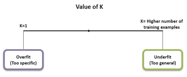
The value of K plays a significant role in the performance efficacy of the model. The chosen K value should neither be too large nor too small. As K increases, the error usually goes down, then stabilizes, and starts rising again when K becomes too large.
If K is too small, the model might perform very well on training data but would drastically fail on testing data (overfitting).
Whereas if K is too large, the resulting model would be too generalized resulting in underfitting. A large K value would also increase the computational expense of your model.
The optimal value of K depends on the dataset being used and largely depends on trial-and-error. Domain knowledge plays a vital role in this.
It is preferable to choose an odd number for K to minimize the chances of landing a tie during class prediction through the majority voting mechanism in KNN classifiers.
More ways that can help with the estimation of the K value are:
- Square Root Method: We can consider the square root of all data points in the training dataset as the optimal value of K.
- Cross-Validation Method: We will start with K=1, run cross-validation (5 to 10-fold), measure the accuracy, and keep repeating until the results get consistent.
- As stated above, as the value of K increases, it stabilizes the error at some point before it rises again. We choose the value at the beginning of the stable zone as the optimal value of K. This is also called Elbow Method.


How to find the K Nearest Neighbors?
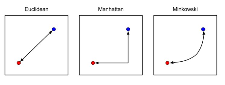
To determine which data points are close enough to be considered nearest neighbors, we commonly use the following distance measuring techniques:
- Euclidean distance (most commonly used method)
- Manhattan distance
- Minkowski distance
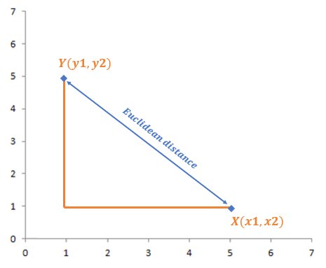
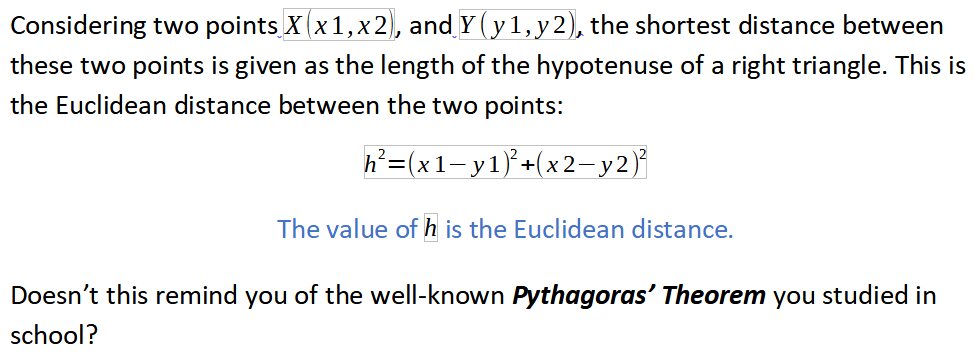
The figure below illustrates how to calculate the Euclidean distance between two points in a 2D space:
How KNN Works?
- Step 1: the optimal value of K is determined.
- Step 2: The KNN algorithm calculates the distance of all data points from the query data point using the distance measuring techniques stated above.
- Step 3: It ranks the data points by increasing distance. The closest K points in the data space of the query point are its nearest neighbors.
- Step 4: For each query point, one of these K neighbors predicts its class as follows.
- Counting the data points in each category and taking the majority votes into consideration – KNN Classifier model.
- Calculating the average of the nearest neighbors – KNN Regressor model.
- Calculating the average of the nearest neighbors – KNN Regressor model.
Building a KNN Classifier in Python
Problem Statement:
For demonstration, we are going to build a classifier model using a K Nearest Neighbors algorithm to predict whether the patients have diabetes or not based on the features in the given data. We will also find the optimal value of K using the GridSearchCV() method in the Scikit-learn library.
So, let’s understand!
Dataset Description:
The dataset has 8 features as given below:
- Pregnancies: Number of times pregnant
- Glucose: Plasma glucose concentration at 2 hours in an oral glucose tolerance test
- BloodPressure: Diastolic blood pressure (mm Hg)
- SkinThickness: Triceps skin fold thickness (mm)
- Insulin: 2-Hour serum insulin (mu U/ml)
- BMI: Body mass index
- DiabetesPedigreeFunction: Diabetes pedigree function
- Age: Age in years
- Outcome: Class variable (0 or 1)
The Outcome column is our target variable.
Tasks to be performed:
- Load the data
- Perform feature scaling
- Perform label encoding
- Split the data into training and testing sets
- Fit the KNN Classifier model
- Generate an accuracy plot
- Create a KNN Classifier with K=7
- Fit the Classifier and get the Accuracy Score
- Create a confusion matrix
- Perform cross-validation
Step 1 – Load the data
\n \n \n <pre class="python" style="font-family:monospace">\n \n \n <span style="color: #808080;font-style: italic">\n \n \n #Import required libraries\n \n \n \n \n \n <span style="color: #ff7700;font-weight:bold">\n \n \n import numpy \n \n \n <span style="color: #ff7700;font-weight:bold">\n \n \n as np\n \n \n \n \n \n <span style="color: #ff7700;font-weight:bold">\n import pandas \n <span style="color: #ff7700;font-weight:bold">\n as pd \n \n <span style="color: #ff7700;font-weight:bold">\n import matplotlib. \n <span style="color: black">\n pyplot \n <span style="color: #ff7700;font-weight:bold">\n as plt \n plt. \n <span style="color: black">\n style. \n <span style="color: black">\n use \n <span style="color: black">\n ( \n <span style="color: #483d8b">\n 'ggplot' \n <span style="color: black">\n ) \n \n \n <span style="color: #808080;font-style: italic">\n #Load the dataset \n data \n <span style="color: #66cc66">\n = pd. \n <span style="color: black">\n read_csv \n <span style="color: black">\n ( \n <span style="color: #483d8b">\n 'diabetes.csv' \n <span style="color: black">\n ) \n data. \n <span style="color: black">\n head \n <span style="color: black">\n ( \n <span style="color: black">\n ) \n </span style="color: black"> \n </span style="color: black"> \n </span style="color: black"> \n </span style="color: black"> \n </span style="color: #483d8b"> \n </span style="color: black"> \n </span style="color: black"> \n </span style="color: #66cc66"> \n </span style="color: #808080;font-style: italic"> \n </span style="color: black"> \n </span style="color: #483d8b"> \n </span style="color: black"> \n </span style="color: black"> \n </span style="color: black"> \n </span style="color: #ff7700;font-weight:bold"> \n </span style="color: black"> \n </span style="color: #ff7700;font-weight:bold"> \n </span style="color: #ff7700;font-weight:bold"> \n </span style="color: #ff7700;font-weight:bold">\n \n \n </span style="color: #ff7700;font-weight:bold">\n \n \n </span style="color: #ff7700;font-weight:bold">\n \n \n </span style="color: #808080;font-style: italic">\n \n \n </pre class="python" style="font-family:monospace">
Step 2 – Perform feature scaling
We will use StandardScaler() to perform the task of Standardization to have a common scale while building our classifier:
\n \n \n <pre class="python" style="font-family:monospace">\n \n \n <span style="color: #ff7700;font-weight:bold">\n \n \n from sklearn.\n \n \n <span style="color: black">\n \n \n preprocessing \n \n \n <span style="color: #ff7700;font-weight:bold">\n \n \n import StandardScaler\n \n \n \n \n \n \n \n \n <span style="color: #808080;font-style: italic">\n #Perform feature scaling \n sc_X \n <span style="color: #66cc66">\n = StandardScaler \n <span style="color: black">\n ( \n <span style="color: black">\n ) \n X \n <span style="color: #66cc66">\n = pd. \n <span style="color: black">\n DataFrame \n <span style="color: black">\n (sc_X. \n <span style="color: black">\n fit_transform \n <span style="color: black">\n (data. \n <span style="color: black">\n drop \n <span style="color: black">\n ( \n <span style="color: black">\n [ \n <span style="color: #483d8b">\n 'Outcome' \n <span style="color: black">\n ] \n <span style="color: #66cc66">\n ,axis \n <span style="color: #66cc66">\n = \n <span style="color: #ff4500">\n 1 \n <span style="color: black">\n ). \n <span style="color: black">\n values \n <span style="color: black">\n ) \n <span style="color: black">\n ) \n y \n <span style="color: #66cc66">\n = data \n <span style="color: black">\n [ \n <span style="color: #483d8b">\n 'Outcome' \n <span style="color: black">\n ]. \n <span style="color: black">\n values \n </span style="color: black"> \n </span style="color: black"> \n </span style="color: #483d8b"> \n </span style="color: black"> \n </span style="color: #66cc66"> \n </span style="color: black"> \n </span style="color: black"> \n </span style="color: black"> \n </span style="color: black"> \n </span style="color: #ff4500"> \n </span style="color: #66cc66"> \n </span style="color: #66cc66"> \n </span style="color: black"> \n </span style="color: #483d8b"> \n </span style="color: black"> \n </span style="color: black"> \n </span style="color: black"> \n </span style="color: black"> \n </span style="color: black"> \n </span style="color: black"> \n </span style="color: black"> \n </span style="color: #66cc66"> \n </span style="color: black"> \n </span style="color: black"> \n </span style="color: #66cc66"> \n </span style="color: #808080;font-style: italic">\n \n \n </span style="color: #ff7700;font-weight:bold">\n \n \n </span style="color: black">\n \n \n </span style="color: #ff7700;font-weight:bold">\n \n \n </pre class="python" style="font-family:monospace">
Step 3 – Perform label encoding
We will use LabelEncoder() to convert the target variable class labels into a numeric form so they become machine-readable:
\n \n \n <pre class="python" style="font-family:monospace">\n \n \n <span style="color: #ff7700;font-weight:bold">\n \n \n from sklearn.\n \n \n <span style="color: black">\n \n \n preprocessing \n \n \n <span style="color: #ff7700;font-weight:bold">\n \n \n import LabelEncoder\n \n \n \n \n \n \n \n \n <span style="color: #808080;font-style: italic">\n #Perform label encoding \n le \n <span style="color: #66cc66">\n = LabelEncoder \n <span style="color: black">\n ( \n <span style="color: black">\n ) \n y \n <span style="color: #66cc66">\n = le. \n <span style="color: black">\n fit_transform \n <span style="color: black">\n (y \n <span style="color: black">\n ) \n </span style="color: black"> \n </span style="color: black"> \n </span style="color: black"> \n </span style="color: #66cc66"> \n </span style="color: black"> \n </span style="color: black"> \n </span style="color: #66cc66"> \n </span style="color: #808080;font-style: italic">\n \n \n </span style="color: #ff7700;font-weight:bold">\n \n \n </span style="color: black">\n \n \n </span style="color: #ff7700;font-weight:bold">\n \n \n </pre class="python" style="font-family:monospace">
Step 4 – Split the data into training and testing sets
We will split the data into 70% training and 30% testing sets:
\n \n \n <pre class="python" style="font-family:monospace">\n \n \n <span style="color: #ff7700;font-weight:bold">\n \n \n from sklearn.\n \n \n <span style="color: black">\n \n \n model_selection \n \n \n <span style="color: #ff7700;font-weight:bold">\n \n \n import train_test_split\n \n \n \n \n \n \n \n \n <span style="color: #808080;font-style: italic">\n #Splitting the Data into Training and Testing Dataset \n X_train \n <span style="color: #66cc66">\n , X_test \n <span style="color: #66cc66">\n , y_train \n <span style="color: #66cc66">\n , y_test \n <span style="color: #66cc66">\n = train_test_split \n <span style="color: black">\n (X \n <span style="color: #66cc66">\n ,y \n <span style="color: #66cc66">\n ,test_size \n <span style="color: #66cc66">\n = \n <span style="color: #ff4500">\n 0.3 \n <span style="color: #66cc66">\n ,random_state \n <span style="color: #66cc66">\n = \n <span style="color: #ff4500">\n 42 \n <span style="color: #66cc66">\n , stratify \n <span style="color: #66cc66">\n =y \n <span style="color: black">\n ) \n </span style="color: black"> \n </span style="color: #66cc66"> \n </span style="color: #66cc66"> \n </span style="color: #ff4500"> \n </span style="color: #66cc66"> \n </span style="color: #66cc66"> \n </span style="color: #ff4500"> \n </span style="color: #66cc66"> \n </span style="color: #66cc66"> \n </span style="color: #66cc66"> \n </span style="color: black"> \n </span style="color: #66cc66"> \n </span style="color: #66cc66"> \n </span style="color: #66cc66"> \n </span style="color: #66cc66"> \n </span style="color: #808080;font-style: italic">\n \n \n </span style="color: #ff7700;font-weight:bold">\n \n \n </span style="color: black">\n \n \n </span style="color: #ff7700;font-weight:bold">\n \n \n </pre class="python" style="font-family:monospace">
Step 5 – Fit the KNN Classifier model
\n \n \n <pre class="python" style="font-family:monospace">\n \n \n <span style="color: #ff7700;font-weight:bold">\n \n \n from sklearn.\n \n \n <span style="color: black">\n \n \n neighbors \n \n \n <span style="color: #ff7700;font-weight:bold">\n \n \n import KNeighborsClassifier\n \n \n \n \n \n \n \n \n <span style="color: #808080;font-style: italic">\n #Setup arrays to store training and test accuracies \n neighbors \n <span style="color: #66cc66">\n = np. \n <span style="color: black">\n arange \n <span style="color: black">\n ( \n <span style="color: #ff4500">\n 1 \n <span style="color: #66cc66">\n , \n <span style="color: #ff4500">\n 9 \n <span style="color: black">\n ) \n train_accuracy \n <span style="color: #66cc66">\n =np. \n <span style="color: black">\n empty \n <span style="color: black">\n ( \n <span style="color: #008000">\n len \n <span style="color: black">\n (neighbors \n <span style="color: black">\n ) \n <span style="color: black">\n ) \n test_accuracy \n <span style="color: #66cc66">\n = np. \n <span style="color: black">\n empty \n <span style="color: black">\n ( \n <span style="color: #008000">\n len \n <span style="color: black">\n (neighbors \n <span style="color: black">\n ) \n <span style="color: black">\n ) \n \n \n <span style="color: #ff7700;font-weight:bold">\n for i \n <span style="color: #66cc66">\n ,k \n <span style="color: #ff7700;font-weight:bold">\n in \n <span style="color: #008000">\n enumerate \n <span style="color: black">\n (neighbors \n <span style="color: black">\n ): \n \n <span style="color: #808080;font-style: italic">\n #Setup a knn classifier with k neighbors \n knn \n <span style="color: #66cc66">\n = KNeighborsClassifier \n <span style="color: black">\n (n_neighbors \n <span style="color: #66cc66">\n =k \n <span style="color: black">\n ) \n \n \n <span style="color: #808080;font-style: italic">\n #Fit the model \n knn. \n <span style="color: black">\n fit \n <span style="color: black">\n (X_train \n <span style="color: #66cc66">\n , y_train \n <span style="color: black">\n ) \n \n \n <span style="color: #808080;font-style: italic">\n #Compute accuracy on the training set \n train_accuracy \n <span style="color: black">\n [i \n <span style="color: black">\n ] \n <span style="color: #66cc66">\n = knn. \n <span style="color: black">\n score \n <span style="color: black">\n (X_train \n <span style="color: #66cc66">\n , y_train \n <span style="color: black">\n ) \n \n \n <span style="color: #808080;font-style: italic">\n #Compute accuracy on the test set \n test_accuracy \n <span style="color: black">\n [i \n <span style="color: black">\n ] \n <span style="color: #66cc66">\n = knn. \n <span style="color: black">\n score \n <span style="color: black">\n (X_test \n <span style="color: #66cc66">\n , y_test \n <span style="color: black">\n ) \n </span style="color: black"> \n </span style="color: #66cc66"> \n </span style="color: black"> \n </span style="color: black"> \n </span style="color: #66cc66"> \n </span style="color: black"> \n </span style="color: black"> \n </span style="color: #808080;font-style: italic"> \n </span style="color: black"> \n </span style="color: #66cc66"> \n </span style="color: black"> \n </span style="color: black"> \n </span style="color: #66cc66"> \n </span style="color: black"> \n </span style="color: black"> \n </span style="color: #808080;font-style: italic"> \n </span style="color: black"> \n </span style="color: #66cc66"> \n </span style="color: black"> \n </span style="color: black"> \n </span style="color: #808080;font-style: italic"> \n </span style="color: black"> \n </span style="color: #66cc66"> \n </span style="color: black"> \n </span style="color: #66cc66"> \n </span style="color: #808080;font-style: italic"> \n </span style="color: black"> \n </span style="color: black"> \n </span style="color: #008000"> \n </span style="color: #ff7700;font-weight:bold"> \n </span style="color: #66cc66"> \n </span style="color: #ff7700;font-weight:bold"> \n </span style="color: black"> \n </span style="color: black"> \n </span style="color: black"> \n </span style="color: #008000"> \n </span style="color: black"> \n </span style="color: black"> \n </span style="color: #66cc66"> \n </span style="color: black"> \n </span style="color: black"> \n </span style="color: black"> \n </span style="color: #008000"> \n </span style="color: black"> \n </span style="color: black"> \n </span style="color: #66cc66"> \n </span style="color: black"> \n </span style="color: #ff4500"> \n </span style="color: #66cc66"> \n </span style="color: #ff4500"> \n </span style="color: black"> \n </span style="color: black"> \n </span style="color: #66cc66"> \n </span style="color: #808080;font-style: italic">\n \n \n </span style="color: #ff7700;font-weight:bold">\n \n \n </span style="color: black">\n \n \n </span style="color: #ff7700;font-weight:bold">\n \n \n </pre class="python" style="font-family:monospace">
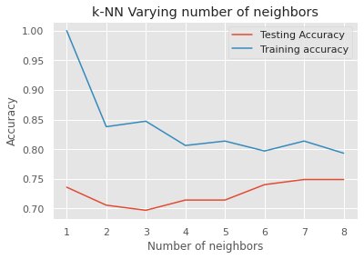
Step 6 – Generate an accuracy plot
\n \n \n <pre class="python" style="font-family:monospace">\n \n \n <span style="color: #808080;font-style: italic">\n \n \n #Generate plot\n \n \n plt.\n \n \n <span style="color: black">\n \n \n title\n \n \n <span style="color: black">\n \n \n (\n \n \n <span style="color: #483d8b">\n 'k-NN Varying number of neighbors' \n <span style="color: black">\n ) \n plt. \n <span style="color: black">\n plot \n <span style="color: black">\n (neighbors \n <span style="color: #66cc66">\n , test_accuracy \n <span style="color: #66cc66">\n , label \n <span style="color: #66cc66">\n = \n <span style="color: #483d8b">\n 'Testing Accuracy' \n <span style="color: black">\n ) \n plt. \n <span style="color: black">\n plot \n <span style="color: black">\n (neighbors \n <span style="color: #66cc66">\n , train_accuracy \n <span style="color: #66cc66">\n , label \n <span style="color: #66cc66">\n = \n <span style="color: #483d8b">\n 'Training accuracy' \n <span style="color: black">\n ) \n plt. \n <span style="color: black">\n legend \n <span style="color: black">\n ( \n <span style="color: black">\n ) \n plt. \n <span style="color: black">\n xlabel \n <span style="color: black">\n ( \n <span style="color: #483d8b">\n 'Number of neighbors' \n <span style="color: black">\n ) \n plt. \n <span style="color: black">\n ylabel \n <span style="color: black">\n ( \n <span style="color: #483d8b">\n 'Accuracy' \n <span style="color: black">\n ) \n plt. \n <span style="color: black">\n show \n <span style="color: black">\n ( \n <span style="color: black">\n ) \n </span style="color: black"> \n </span style="color: black"> \n </span style="color: black"> \n </span style="color: black"> \n </span style="color: #483d8b"> \n </span style="color: black"> \n </span style="color: black"> \n </span style="color: black"> \n </span style="color: #483d8b"> \n </span style="color: black"> \n </span style="color: black"> \n </span style="color: black"> \n </span style="color: black"> \n </span style="color: black"> \n </span style="color: black"> \n </span style="color: #483d8b"> \n </span style="color: #66cc66"> \n </span style="color: #66cc66"> \n </span style="color: #66cc66"> \n </span style="color: black"> \n </span style="color: black"> \n </span style="color: black"> \n </span style="color: #483d8b"> \n </span style="color: #66cc66"> \n </span style="color: #66cc66"> \n </span style="color: #66cc66"> \n </span style="color: black"> \n </span style="color: black"> \n </span style="color: black"> \n </span style="color: #483d8b">\n \n \n </span style="color: black">\n \n \n </span style="color: black">\n \n \n </span style="color: #808080;font-style: italic">\n \n \n </pre class="python" style="font-family:monospace">
From the above plot, we can observe that we get the maximum testing accuracy for K=7 and K=8. As discussed above, we will choose the odd value for K.
So, let’s create a KNeighborsClassifier with the nearest number of neighbors as 7:
Step 8 – Fit the Classifier and get the Accuracy Score
\n \n \n <pre class="python" style="font-family:monospace">\n \n \n <span style="color: #808080;font-style: italic">\n \n \n #Fit the model\n \n \n knn.\n \n \n <span style="color: black">\n \n \n fit\n \n \n <span style="color: black">\n \n \n (X_train\n \n \n <span style="color: #66cc66">\n ,y_train \n <span style="color: black">\n ) \n y_pred \n <span style="color: #66cc66">\n = knn. \n <span style="color: black">\n predict \n <span style="color: black">\n (X_test \n <span style="color: black">\n ) \n \n \n <span style="color: #808080;font-style: italic">\n #Calculating Model Accuracy \n \n <span style="color: #ff7700;font-weight:bold">\n from sklearn. \n <span style="color: black">\n metrics \n <span style="color: #ff7700;font-weight:bold">\n import accuracy_score \n \n <span style="color: #ff7700;font-weight:bold">\n print \n <span style="color: black">\n ( \n <span style="color: #483d8b">\n "Accuracy of test set=" \n <span style="color: #66cc66">\n ,accuracy_score \n <span style="color: black">\n (y_test \n <span style="color: #66cc66">\n , y_pred \n <span style="color: black">\n )* \n <span style="color: #ff4500">\n 100 \n <span style="color: black">\n ) \n </span style="color: black"> \n </span style="color: #ff4500"> \n </span style="color: black"> \n </span style="color: #66cc66"> \n </span style="color: black"> \n </span style="color: #66cc66"> \n </span style="color: #483d8b"> \n </span style="color: black"> \n </span style="color: #ff7700;font-weight:bold"> \n </span style="color: #ff7700;font-weight:bold"> \n </span style="color: black"> \n </span style="color: #ff7700;font-weight:bold"> \n </span style="color: #808080;font-style: italic"> \n </span style="color: black"> \n </span style="color: black"> \n </span style="color: black"> \n </span style="color: #66cc66"> \n </span style="color: black"> \n </span style="color: #66cc66">\n \n \n </span style="color: black">\n \n \n </span style="color: black">\n \n \n </span style="color: #808080;font-style: italic">\n \n \n </pre class="python" style="font-family:monospace">
Step 9 – Create a confusion matrix
A confusion matrix describes the performance of a classifier model on a set of test data for which the true values are known. We will calculate the confusion matrix using the confusion_matrix() method of Scikit-learn:
\n \n \n <pre class="python" style="font-family:monospace">\n \n \n <span style="color: #808080;font-style: italic">\n \n \n #Confusion Matrix\n \n \n confusion_matrix \n \n \n <span style="color: #66cc66">\n \n \n = confusion_matrix\n \n \n <span style="color: black">\n \n \n (y_test\n \n \n <span style="color: #66cc66">\n , y_pred \n <span style="color: black">\n ) \n confusion_matrix \n </span style="color: black"> \n </span style="color: #66cc66">\n \n \n </span style="color: black">\n \n \n </span style="color: #66cc66">\n \n \n </span style="color: #808080;font-style: italic">\n \n \n </pre class="python" style="font-family:monospace">
Considering the obtained confusion matrix, we have:
- True negative = 131
- False positive = 19
- True positive = 42
- False negative = 39
Step 10 – Perform cross-validation
Cross-validation is a technique to evaluate predictive models by dividing the dataset into a training set to train the model, and a test set to evaluate it.
We will be using the Scikit-learn’s function called GridSearchCV i.e., Grid Search cross-validation, as shown:
\n \n \n <pre class="python" style="font-family:monospace">\n \n \n <span style="color: #ff7700;font-weight:bold">\n \n \n from sklearn.\n \n \n <span style="color: black">\n \n \n model_selection \n \n \n <span style="color: #ff7700;font-weight:bold">\n \n \n import GridSearchCV\n \n \n \n \n \n \n \n \n <span style="color: #808080;font-style: italic">\n #In KNN, the parameter to be tuned is n_neighbors \n param_grid \n <span style="color: #66cc66">\n = \n <span style="color: black">\n { \n <span style="color: #483d8b">\n 'n_neighbors':np. \n <span style="color: black">\n arange \n <span style="color: black">\n ( \n <span style="color: #ff4500">\n 1 \n <span style="color: #66cc66">\n , \n <span style="color: #ff4500">\n 50 \n <span style="color: black">\n ) \n <span style="color: black">\n } \n \n knn \n <span style="color: #66cc66">\n = KNeighborsClassifier \n <span style="color: black">\n ( \n <span style="color: black">\n ) \n knn_cv \n <span style="color: #66cc66">\n = GridSearchCV \n <span style="color: black">\n (knn \n <span style="color: #66cc66">\n ,param_grid \n <span style="color: #66cc66">\n ,cv \n <span style="color: #66cc66">\n = \n <span style="color: #ff4500">\n 5 \n <span style="color: black">\n ) \n knn_cv. \n <span style="color: black">\n fit \n <span style="color: black">\n (X \n <span style="color: #66cc66">\n ,y \n <span style="color: black">\n ) \n </span style="color: black"> \n </span style="color: #66cc66"> \n </span style="color: black"> \n </span style="color: black"> \n </span style="color: black"> \n </span style="color: #ff4500"> \n </span style="color: #66cc66"> \n </span style="color: #66cc66"> \n </span style="color: #66cc66"> \n </span style="color: black"> \n </span style="color: #66cc66"> \n </span style="color: black"> \n </span style="color: black"> \n </span style="color: #66cc66"> \n </span style="color: black"> \n </span style="color: black"> \n </span style="color: #ff4500"> \n </span style="color: #66cc66"> \n </span style="color: #ff4500"> \n </span style="color: black"> \n </span style="color: black"> \n </span style="color: #483d8b"> \n </span style="color: black"> \n </span style="color: #66cc66"> \n </span style="color: #808080;font-style: italic">\n \n \n </span style="color: #ff7700;font-weight:bold">\n \n \n </span style="color: black">\n \n \n </span style="color: #ff7700;font-weight:bold">\n \n \n </pre class="python" style="font-family:monospace">
knn_cv.best_score_
knn_cv.best_params_
So, our KNN classifier with 17 nearest neighbors achieves the best accuracy score of about 76%.
Pros and Cons of KNN
Pros –
- Simple and intuitive algorithm.
- It is a non-parametric algorithm which means it does not need any assumptions to implement.
- Evolves constantly which allows the algorithm to respond quickly to real-time input changes.
- Works well with multiclass data in classification problems.
- Works equally well with regression problems.
- We can use it to implement non-linear tasks.
Cons –
- It is a slow algorithm.
- Sensitive to outliers.
- Suffers from the curse of dimensionality
- The dataset should have homogenous features for the algorithm to predict accurately.
- No capability to deal with missing values in the data.


Conclusion
The KNN algorithm in machine learning is a simple, yet versatile supervised algorithm that can be used to solve both classification and regression problems. Machine learning & intelligence are rapidly growing areas in the IT industry and have a huge impact on big businesses across the globe.
Top Trending Articles:
Data Analyst Interview Questions | Data Science Interview Questions | Machine Learning Applications | Big Data vs Machine Learning | Data Scientist vs Data Analyst | How to Become a Data Analyst | Data Science vs. Big Data vs. Data Analytics | What is Data Science | What is a Data Scientist | What is Data Analyst
This is a collection of insightful articles from domain experts in the fields of Cloud Computing, DevOps, AWS, Data Science, Machine Learning, AI, and Natural Language Processing. The range of topics caters to upski... Read Full Bio


