Least Square Regression in Machine Learning
This article discusses the concept of linear regression. We have also covered least square regression in machine learning. Let’s begin!
Least Square Regression is a statistical method commonly used in machine learning for analyzing and modelling data. It involves finding the line of best fit that minimizes the sum of the squared residuals (the difference between the actual values and the predicted values) between the independent variable(s) and the dependent variable.
We can use Least Square Regression for both simple linear regression, where there is only one independent variable. Also, for multiple linear regression, where there are several independent variables. We widely use this method in a variety of fields, such as economics, engineering, and finance, to model and predict relationships between variables. Before learning least square regression, let’s understand linear regression.
Linear Regression
Linear regression is one of the basic statistical techniques in regression analysis. People use it for investigating and modelling the relationship between variables (i.e. dependent variable and one or more independent variables).
Before being promptly adopted into machine learning and data science, linear models were used as basic statistical tools to assist prediction analysis and data mining. If the model involves only one regressor variable (independent variable), it is called simple linear regression, and if the model has more than one regressor variable, the process is called multiple linear regression.
Equation of Straight Line
Let’s consider a simple example of an engineer wanting to analyze vending machines' product delivery and service operations. He/she wants to determine the relationship between the time required by a deliveryman to load a machine and the volume of the products delivered. The engineer collected the delivery time (in minutes) and the volume of the products (in a number of cases) of 25 randomly selected retail outlets with vending machines. The scatter diagram is the observations plotted on a graph.
Now, if I consider Y as delivery time (dependent variable), and X as product volume delivered (independent variable). Then we can represent the linear relationship between these two variables as
Okay! Now that looks familiar. Its equation is for a straight line, where m is the slope and c is the y-intercept. Our objective is to estimate these unknown parameters in the regression model such that they give minimal error for the given dataset. Commonly referred to as parameter estimation or model fitting. In machine learning, the most common method of estimation is the Least Squares method.
Best-suited Machine Learning courses for you
Learn Machine Learning with these high-rated online courses
What is the Least Square Regression Method?
Least squares is a commonly used method in regression analysis for estimating the unknown parameters by creating a model which will minimize the sum of squared errors between the observed data and the predicted data.
Basically, it is one of the widely used methods of fitting curves that works by minimizing the sum of squared errors as small as possible. It helps you draw a line of best fit depending on your data points.
Finding the Line of Best Fit Using Least Square Regression
Given any collection of a pair of numbers and the corresponding scatter graph, the line of best fit is the straight line that you can draw through the scatter points to represent the relationship between them best. So, back to our equation of the straight line, we have:
Where,
Y: Dependent Variable
m: Slope
X: Independent Variable
c: y-intercept
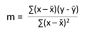
Our aim here is to calculate the values of slope y-intercept and substitute them in the equation along with the values of independent variable X to determine the values of dependent variable Y. Let’s assume that we have ‘n’ data points, then we can calculate slope using the scary looking formula below:
Then, the y-intercept is calculated using the formula:
Lastly, we substitute these values in the final equation Y = mX + c. Simple enough, right? Now let’s take a real-life example and implement these formulas to find the line of best fit.
Least Squares Regression Example
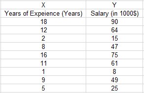
Let us take a simple dataset to demonstrate the least squares regression method.
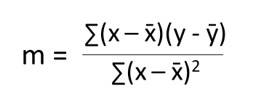
Step 1: The first step is to calculate the slope ‘m’ using the formula
After substituting the respective values in the formula, m = 4.70 approximately.
Step 2: Next, calculate the y-intercept ‘c’ using the formula (ymean — m * xmean). By doing that, the value of c approximately is c = 6.67.
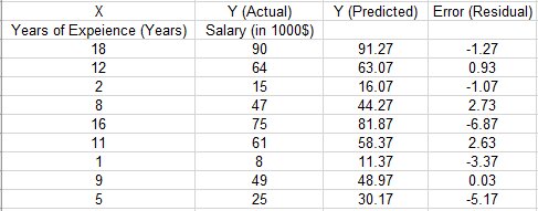
Step 3: Now we have all the information needed for the equation, and by substituting the respective values in Y = mX + c, we get the following table. Using this information, you can now plot the graph.
This way, the least squares regression method provides the closest relationship between the dependent and independent variables by minimizing the distance between the residuals (or error) and the trend line (or line of best fit). Therefore, the sum of squares of residuals (or error) is minimal under this approach.
Now let us master how the least squares method is implemented using Python.
Least Squares Regression in Python
Scenario
A rocket motor is manufactured by combining an igniter propellant and a sustainer propellant inside a strong metal housing. It was noticed that the shear strength of the bond between two propellers is strongly dependent on the age of the sustainer propellant.
Problem Statement
Implement a simple linear regression algorithm using Python to build a machine-learning model that studies the relationship between the shear strength of the bond between two propellers and the age of the sustainer propellant.
Let’s begin!
Steps
Step 1: Import the required Python libraries.
# Importing Librariesimport numpy as npimport pandas as pdimport matplotlib.pyplot as plt
Step 2: Next step is to read and load the dataset that we are working on.
# Loading datasetdata = pd.read_csv('PropallantAge.csv')data.head()data.info()
This gives you a preview of your data and other related information that’s good to know. Our aim now is to find the relationship between the age of sustainer propellant and the shear strength of the bond between two propellers.
Step 3 (optional): You can create a scatter plot just to check the relationship between these two variables.
# Plotting the dataplt.scatter(data['Age of Propellant'],data['Shear Strength'])
Step 4: The next step is to assign X and Y as independent and dependent variables, respectively.
# Computing X and YX = data['Age of Propellant'].valuesY = data['Shear Strength'].values
Step 5: As we calculated manually earlier, we need to compute the mean of variables X and Y to determine the values of slope (m) and y-intercept. Also, let n be the total number of data points.
# Mean of variables X and Ymean_x = np.mean(X)mean_y = np.mean(Y) # Total number of data valuesn = len(X)
Step 6: In the next step, we will calculate the slope and the y-intercept using the formulas we discussed above.
# Calculating 'm' and 'c'num = 0denom = 0for i in range(n): num += (X[i] - mean_x) * (Y[i] - mean_y) denom += (X[i] - mean_x) ** 2m = num / denomc = mean_y - (m * mean_x) # Printing coefficientsprint("Coefficients")print(m, c)
The above step has given us the values of m and c. Substituting them, we get,
Shear Strength = 2627.822359001296 + (-37.15359094490524) * Age of Propellant
Step 7: The above equation represents our linear regression model. Now, let’s plot this graphically.
# Plotting Values and Regression Line maxx_x = np.max(X) + 10minn_x = np.min(X) - 10 # line values for x and yx = np.linspace(minn_x, maxx_x, 1000)y = c + m * x # Ploting Regression Lineplt.plot(x, y, color='#58b970', label='Regression Line') # Ploting Scatter Pointsplt.scatter(X, Y, c='#ef5423', label='Scatter Plot') plt.xlabel('Age of Propellant (in years)')plt.ylabel('Shear Strength')plt.legend()plt.show()
Output:
Well! That’s it! We successfully found the line of best fit and fitted it into the data points using the least square regression method in machine learning. So, now, using this, I could verify that there is a strong statistical relationship between the shear strength and the propellant age.
Run this demo in Colab – Try it yourself

Conclusion
So, you found the curve of best fit? Now what? After obtaining the least-squares fit, a number of intriguing questions pop up, such as:
- How well does the equation that you found fit the data?
- Will this linear model be useful as a predictor in real time?
- Also, where assumptions are violated, such as uncorrelated errors, constant variance, etc. If yes, how serious is the effect?
- And many more….
We should consider all of these issues before adopting the model.
So, we hope this article on least square regression in machine learning helped you to understand the concepts.
Contributed By: Varun Dwarki
This is a collection of insightful articles from domain experts in the fields of Cloud Computing, DevOps, AWS, Data Science, Machine Learning, AI, and Natural Language Processing. The range of topics caters to upski... Read Full Bio


